1 Installing R on your machine

To download and install R for the first time you can go the webpage:

http://cran.r-project.org

Select the platform for your machine (i.e. Windows) and select: install R for the first time. Thereafter, select the latest version of the software and install as you would for any other program. If you are making use of a linux operating system then go to https://cran.r-project.org/bin/linux/, select your distribution (i.e. debian, redhat, suse, or ubuntu) and follow the instructions that are provided.

While the base R software comes with a GUI, it is very basic and not ideal for someone who is starting out. As such we are going to make use of the RStudio integrated development environment (IDE), which can be downloaded for free at:

http://www.rstudio.com

To select the download the user interface go to the RStudio website and select the appropriate options to download the desktop version of this software. After you have installed this software, you will then be able to gain access to the wonderful world of R through the RStudio application.

While RStudio is possibly the most popular IDE for R, you may wish to make use of generic IDE’s such as Virtual Studio, Atom, Sublime Text, Kate, Notepad ++, or Vim. These are all pretty useful if you are simultaneously coding in different software languages, or if you want to make use of a single environment to do your modelling and description of the model (although there are now better ways of doing this within the R programming environment).

In addition to these two programs, I would also recommend that Windows users should download and install the Rtools program, which is available at:

https://cran.r-project.org/bin/windows/Rtools/

Apple mac users should consider installing the Xcode command line tools, which are available at:

https://developer.apple.com/downloads

Linux users should install the R development package, usually called r-devel or r-base-dev.

This will allow you to interface with GitLab or GitHub accounts and would allow you to gain access to many other interesting aspects of this programming language.

2 Resources

You can find helpful tutorials by following CRAN’s link to Contributed Documentation. If you are new to this language, then Paradis (2005) is a great introduction. The English version can be download from the CRAN website:

http://cran.r-project.org/doc/contrib/Paradis-rdebuts_en.pdf

More recently, there are also a number of online courses that provide a great introduction. For example, you may wish to take a look at:

https://www.datacamp.com/courses/free-introduction-to-r

Or alternatively, all UCT staff and students can access the online training material at https://www.linkedin.com/learning at no charge, where you may want to consider taking the courses:

https://www.linkedin.com/learning/learning-r/welcome?u=70295562

https://www.linkedin.com/learning/r-statistics-essential-training/welcome?u=70295562

https://www.linkedin.com/learning/data-science-foundations-fundamentals/exercise-files?u=70295562

Other options include teaching yourself R with the aid of the swirl package that has been written in R. Details of this package can be found at:

http://swirlstats.com/

For those who would like to invest more time on programming, then you could take a look at the text by Wickham (2014). In addition, his website is particularly good and his GitHub repository includes a few GitBook’s that are worth reading. One of which is the text:

http://adv-r.had.co.nz/

He is also the author of the tidyverse, which is the main package for data wrnagling and visualisation. You can check out details of this at: https://www.tidyverse.org/.

The academic publisher Springer has released an inexpensive and focused series of books, titled Use R!, which discuss the use of R in a various subject areas. The series now includes over 65 titles and they all contain source code, which I have found these to be extremely useful. You can find these titles at:

http://www.springer.com/series/6991?detailsPage=titles

The publisher CRC Press (which is part of the Taylor & Francis Group) have a similar series of books, which may be viewed at:

https://www.crcpress.com/Chapman--HallCRC-The-R-Series/book-series/CRCTHERSER

A further useful resource is the Journal of Statistical Software, which contains journal articles that seek to explain many of the packages that are available on the R website. These articles are usually similar to the vignettes that accompany most packages.

For a list of the major econometric type of packages, including those that have been developed for time series, microeconometric and panel models, see the websites:

http://cran.r-project.org/web/views/Econometrics.html

https://cran.r-project.org/web/views/TimeSeries.html

https://cran.r-project.org/web/views/Finance.html

If you are also interested in computational issues, then you may wish to visit the webpages:

https://cran.r-project.org/web/views/NumericalMathematics.html

https://cran.r-project.org/web/views/HighPerformanceComputing.html

Alternatively for the complete set of the package categories:

https://cran.r-project.org/web/views/

Or you can find all the packages that have been sorted by name at:

http://cran.r-project.org/web/packages/available_packages_by_name.html

Remember also that the total number of packages on the CRAN repository represent only a small fraction of those that are available. So if you don’t find what you like on this particular repository then it may be available elsewhere, possibly on a GitHub or GitLab repository, you just need to search.

In addition, if you are struggling with a particular function in R, then you may want to check out the StackOverFlow webpage, which was originally developed for computer programmers (many of which make use of R for data science applications). The probability that your query has been previously answered is usually quite high and what is particularly nice about this website is that it has a number of methods that avoid the duplication of queries. You can check it out at:

http://stackoverflow.com/

Then lastly, as most of my programming experience has been obtained in Matlab, I have also found the text by Hiebeler (2015) to be of use. He has a particularly nice summary document that can be found at:

http://www.math.umaine.edu/~hiebeler/comp/matlabR.pdf

Similar documentation can be found for those who may be more familiar with Python or Julia.¹ Unfortunately, I have not found anything that is all that good for Stata users, as the Stata environment is somewhat different to that of most other scripting languages. However, I can tell you that some of the Stata users that I’ve worked with have found the transition to R to be relatively straightfoward. Those who are interested may find the book by Muenchen and Hilbe (2010) to be of use, although it is not a quick read.² If you are interested in using Python for econometrics then check out the website of Kevin Shepphard at:

https://www.kevinsheppard.com

In addition, if you want to use either Python or Julia for applications in mathematical economics then check out the website of Thomas Sargent and John Stachurski at:

http://quant-econ.net

3 Desktop Overview

After you have installed the software that has been mentioned above, you will be able to open RStudio. When making use of this software, it would look similar to that which is shown in Figure 1.

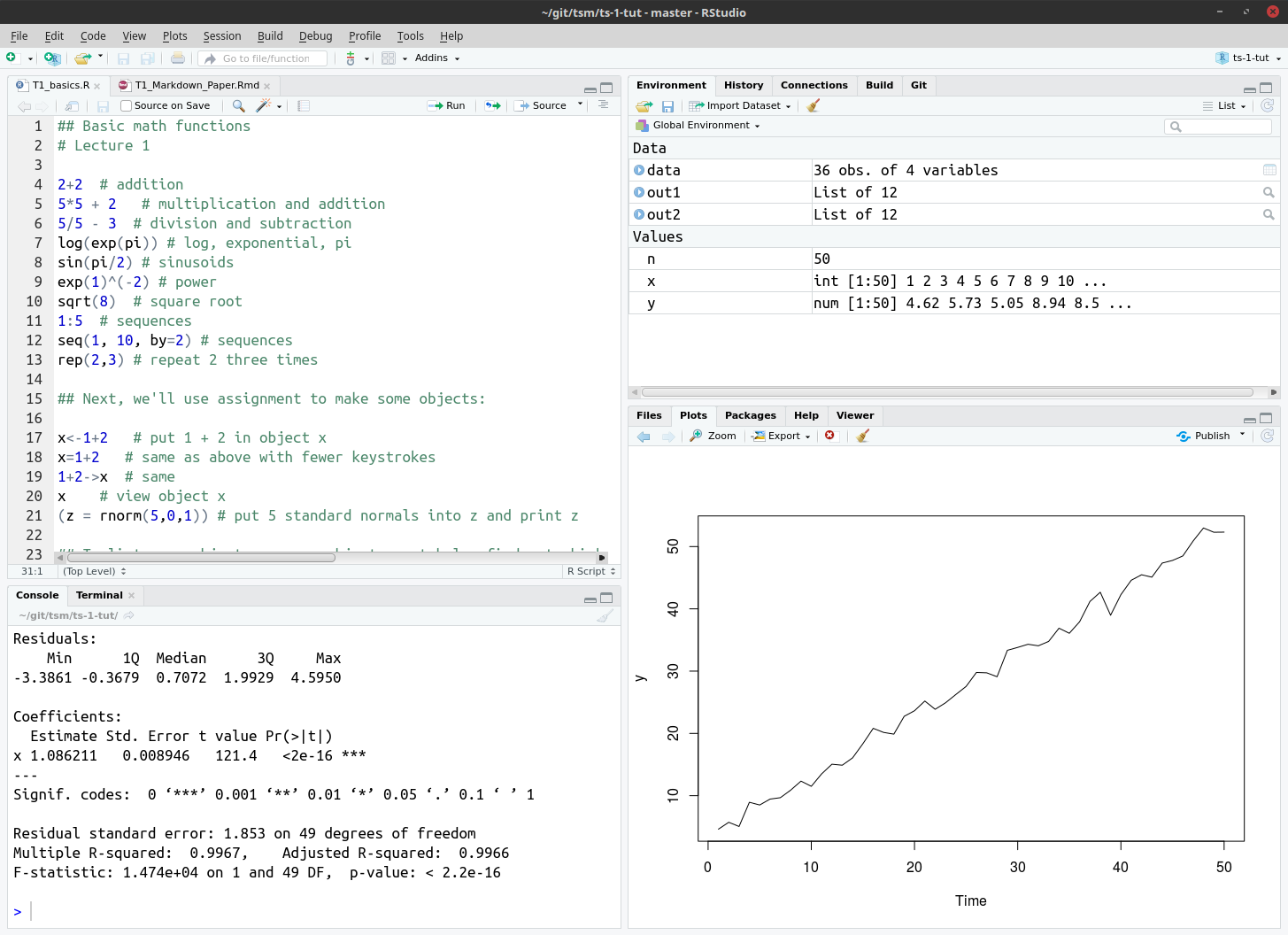
• The basic program file (what Stata users call do files) is usually displayed in the top left-hand corner. One is able to view multiple program files at once and you can also execute entire files, single lines or just a subset of a line.
• All the variables, matrices, scalars, objects, strings, etc. are store in the Environment on the top right.
• Any conceivable type of graph may be constructed and displayed in the Plots panel on the bottom right. These may be exported as jpeg’s, pdf’s, etc.
• The Console on the bottom left may be used to input commands or provide output (which may be structured to your liking).
• If you double-click on a Data element in the Environment it will display it in a Excel type screen on the left panel.
• The additional tabs on the bottom right contain additional useful information. Screen shots of these are contained below.
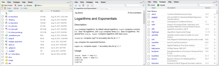
• The Files directory takes on a Windows Explorer type of interface, which allows you to negotiate your way around your current directory.
• There is a very useful Help function that provides the exact format for the respective commands. It will also contain an example of it’s use as well as textbook/journal references (where appropriate).
• To install and use Packages you can use the respective tab, which will link you to the repository on the web. When you click on the package name you will see all the available functions in the package. In addition, some packages will include a very useful vignette, which is an equivalent of a journal article that explains the methodology and application of the package. It will also include a working example with code (in most cases).

4 Basic overview of programming in R

#> Basic commands: ----

2 + 2     # addition

## [1] 4

5*5 + 2   # multiplication and addition

## [1] 27

5/5 - 3   # division and subtraction

## [1] -2

log(exp(pi))  # log, exponential, pi

## [1] 3.141593

sin(pi/2) # sinusoids

## [1] 1

exp(1)^(-2)   # power

## [1] 0.1353353

sqrt(8)   # square root

## [1] 2.828427

1:5   # sequences

## [1] 1 2 3 4 5

seq(1, 10, by=2) # sequences

## [1] 1 3 5 7 9

rep(2,3)  # repeat 2 three times

## [1] 2 2 2

#> Assign values to objects: ----
x <- 1 + 2   # put 1 + 2 in object x
x = 1 + 2    # same as above with fewer keystrokes
x    # view object x

## [1] 3

(z = rnorm(5,0,1)) # put 5 standard normals into z and print

## [1]  0.7241835 -1.1344268  0.7276477 -1.3847352
## [5] -1.6150733

#> List objects, get help and get current working directory: ----
ls()   # list all objects

## [1] "figs" "tbls" "x"    "z"

help(exp)   # specific help (?exp is the same)
getwd()    # get working directory (tells you where R is pointing)

## [1] "/home/kevin/git/tsm/ts-1-tut"

#> Set working directory and quit: ----
setwd('C://Users')   # change working directory (note double slash)
q()   # end the session (keep reading)

#> To create your own data set: ----
mydata = c(1,2,3,2,1)  # where we concatenated the numbers
mydata  # display the data

## [1] 1 2 3 2 1

mydata[3]  # the third element

## [1] 3

mydata[3:5]   # elements three through five

## [1] 3 2 1

mydata[-(1:2)]   # everything except the first two elements

## [1] 3 2 1

length(mydata)  # length of elements

## [1] 5

mydata = as.matrix(mydata) # make it a matrix
dim(mydata)  # provide dimensions of matrix

## [1] 5 1

#> Rules for doing arithmetic with vectors: ----
x=c(1,2,3,4); y=c(2,4,6,8); z=c(10,20) # three commands are stacked with ;
x*y   # i.e. 1*2, 2*4, 3*6, 4*8

## [1]  2  8 18 32

x/z   # i.e. 1/10, 2/20, 3/10, 4/20

## [1] 0.1 0.1 0.3 0.2

x+z   # i.e. 1+10, 2+20, 3+10, 4+20

## [1] 11 22 13 24

x %*% y  # matrix multiplication

##      [,1]
## [1,]   60

#> Basic loops: ----

for (id1 in 1:4){
  print(paste("Execute model number", id1))
}  # for loops are the most common

## [1] "Execute model number 1"
## [1] "Execute model number 2"
## [1] "Execute model number 3"
## [1] "Execute model number 4"

id2 <- 1
while (id2 < 6) {
  print(id2)
  id2 = id2 + 1
}  # while loops can be used as an alternative

## [1] 1
## [1] 2
## [1] 3
## [1] 4
## [1] 5

x <- -5  # use else statement to test if this is positive or negative

if (x == 0) {
  print("Zero")
} else if (x > 0) {
  print("Positive number")
} else {
  print("Negative number")
}

## [1] "Negative number"

# Could also vectorise code and use `sapply or `tidyverse::map` function to make code run quicker

#> Simulating regression data: ----
n <- 50 # number of observations
x <- seq(1, n) # right-hand side variable
y <- 3 + x + rnorm(n) # left-hand side variable

plot(x, y) # show the linear relationship between the variables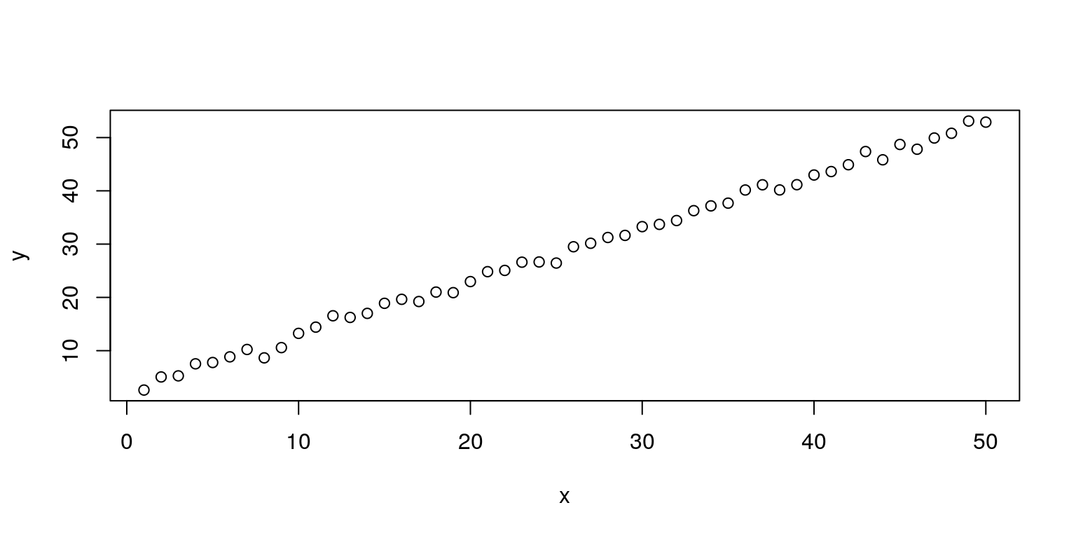

plot.ts(y) # plot time series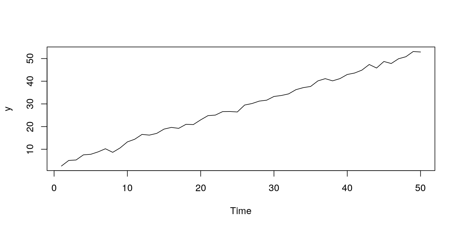

#> Estimate a linear regression model: ----
out1 <- lm(y ~ x- 1) # regress x on y without constant
summary(out1) # generate output

## 
## Call:
## lm(formula = y ~ x - 1)
## 
## Residuals:
##     Min      1Q  Median      3Q     Max 
## -3.5994 -0.3817  1.1129  1.7931  5.0407 
## 
## Coefficients:
##   Estimate Std. Error t value Pr(>|t|)    
## x 1.087158   0.009542   113.9   <2e-16 ***
## ---
## Signif. codes:  
## 0 '***' 0.001 '**' 0.01 '*' 0.05 '.' 0.1 ' ' 1
## 
## Residual standard error: 1.977 on 49 degrees of freedom
## Multiple R-squared:  0.9962, Adjusted R-squared:  0.9962 
## F-statistic: 1.298e+04 on 1 and 49 DF,  p-value: < 2.2e-16

#> Working with real data: ----
rm(list=ls()) # clear data
graphics.off() # close graphs

setwd('C:\\TimeSeries\\1_Intro\\tut')

data <- read.csv(file="data.csv") # read in csv data

out2 <- lm(data$y ~ data$k) # estimation a linear regression
summary(out2) # generate output

## 
## Call:
## lm(formula = data$y ~ data$k)
## 
## Residuals:
##      Min       1Q   Median       3Q      Max 
## -0.51371 -0.23632  0.06197  0.25068  0.40872 
## 
## Coefficients:
##             Estimate Std. Error t value Pr(>|t|)    
## (Intercept)  0.63668    0.09998   6.368 2.88e-07 ***
## data$k      -0.14167    0.17601  -0.805    0.426    
## ---
## Signif. codes:  
## 0 '***' 0.001 '**' 0.01 '*' 0.05 '.' 0.1 ' ' 1
## 
## Residual standard error: 0.3093 on 34 degrees of freedom
## Multiple R-squared:  0.0187, Adjusted R-squared:  -0.01016 
## F-statistic: 0.6479 on 1 and 34 DF,  p-value: 0.4265

# clear data & close graphs
rm(list=ls())
graphics.off()

5 Loading data

The easiest way to import data into R is to make use of a .csv file format from an Excel spredsheet. You can take a look at the existing datafiles that I use in the tutorials to get an idea of the suggested format. Note that I use columns for the data and would give the column a name in the first cell of the column.

Once you have your data as you want it in Excel you need to then save it. Choose the option to File > Save As, then under the type of file, change the Excel Workbook (.xlsx) to CSV (Comma delimited)(.csv). In this example, I have called my data file data.csv.

Now you can go to RStudio, where you will see in each program file I would always clear the data and close the plots with the following commands.

rm(list=ls())   # clear data
graphics.off()  # close graphs

Thereafter, it is a good idea to specify a working directory, which would be where you data file is located.

setwd('C:\\TimeSeriesAnalysis\\1_Intro\\tut')

The next part would then be to import the data with the use of read.csv command. In this case, we create an object called data that will have the column names for each of the time series variables.

data <- read.csv(file="data.csv")   # read in csv data

In some versions of Windows (notably Windows 8) it saves a .csv file with semi-comma separators, in which case you would need to change the above command to:

  data <- read.csv(file="data.csv", sep=";")  # read in csv data

Remember also that you need to make sure that the variable has been correctly loaded by plotting the data. In some instances the data may be imported as a logical operator or as a factor. To plot the data make use of the command:

plot.ts(data$y)   # plot time series

where the variable in our Excel datafile would have been labelled as y. If it looks incorrect then you can always convert the variable into a numeric field using the command:

data.tmp <- as.numeric(data$y)

In this case the new variable would be called data.tmp. As an alternative to using these commands, you can just use the Import Dataset button on the Environment tab and it will take you through the necessary steps.

6 Other aspects of interest

library("devtools")
install_github("username/packagename")

devtools::install_github("username/packagename")

install.packages("C:\\GitHub\\ggplot2", repos=NULL, type="source")

.libPaths()

update.packages()

7 Concluding Comments

During the course of this semester we are really only going to touch the surface of what is possible in this programming environment. For those of you that want to explore the data-organising capabilities, then start by taking a look at the tidyverse package for data wrangling and if you need to interact with a large database, the RODBC package is simple to use and works nicely. If you are working with time series data that has strange frequencies then the zoo or xts packages are particularly useful. For working with time series data the lubridate and tibbletime packages allow us to manipulate large datasets with relative ease.

In addition, if you want to make attractive figures for your research then the ggplot2 package should be a good first port of call. And if you want to make use of an interactive website then the shiny package has impressive functionality. And then there are any number of statistical and machine learning packages that could be used for most forms of analysis.

8 References