Tutorial: Simulating and Estimating ARMA models
by Kevin Kotzé
1 Basic setup for most empirical work
To have a look at the first program for this session, please open the file T2_arma.R. After providing a brief description of what this program seeks to achieve, the first thing that we usually do is clear all variables from the current environment and close all the plots. This is performed with the following commands:
rm(list = ls())  # clear all variables in workspace
graphics.off()  # clear all plots
Thereafter, we will load the toolboxes that we need for this session. There are a few routines that I’ve compiled in a package that is contained on my GitHub account. To install this package, which is named tsm you need to run the following commands:
devtools::install_github("KevinKotze/tsm")
devtools::install_github("cran/fArma")
The next step is to make sure that you can access the routines in this package by making use of the library command.
library(tsm)2 Simulated autoregressive process
Now we are good to go! Let’s generate 1000 observations for a simulated AR(1) time series process with \(\phi = 0.8\). To ensure that we all get the same results, we set the seed to a predetermined value before we generate values for the respective variable, which has been assigned the name of \(x\).
set.seed(123)
x <- arima.sim(model = list(ar = 0.8), n = 1000)
To plot the time series we can use the plot.ts, which is quick and easy to use. Thereafter, we can take a look at autocorrelation and partial autocorrelation function for this variable using the ac command.
plot.ts(x)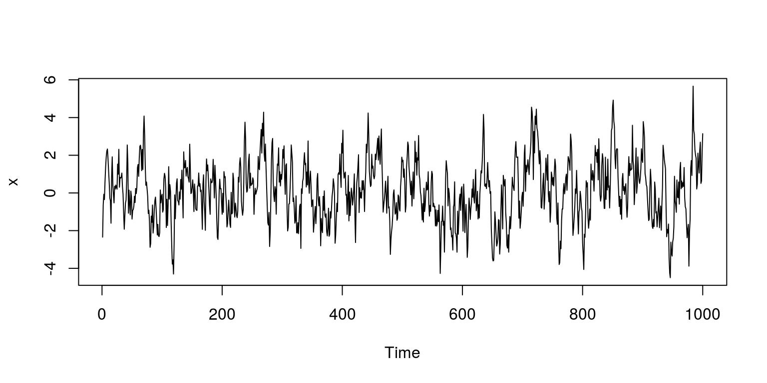
ac(x, max.lag = 18)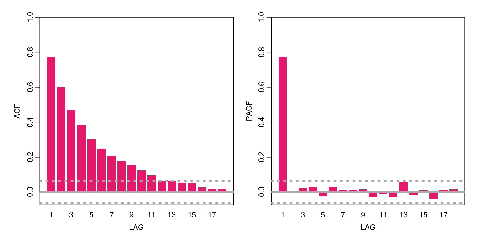
To display the Ljung-Box statistic for the first lag we would execute the command, where we note that the p-value suggests that the autocorrelation is different from zero.
Box.test(x, lag = 1, type = "Ljung-Box")##
## Box-Ljung test
##
## data: x
## X-squared = 599.78, df = 1, p-value < 2.2e-16Similarly, we could assign the output from the test to an object Box.res.
Box.res <- Box.test(x, lag = 1, type = "Ljung-Box")To check what is in the object Box.res we could just type:
Box.res##
## Box-Ljung test
##
## data: x
## X-squared = 599.78, df = 1, p-value < 2.2e-16Or alternatively you could use print(Box.res). If we then want to create a vector of Q-stats for the first 10 lags we can assign values to a object we would create a vector for the Q-stat results
Q.stat <- rep(0, 10)  # creates a vector for ten observations, where 0 is repeated 10 times
Q.prob <- rep(0, 10)
Thereafter, we assign values for the Q-stat to element places in the different objects. For the first statistic:
Q.stat[1] <- Box.test(x, lag = 1, type = "Ljung-Box")$statistic
Q.prob[1] <- Box.test(x, lag = 1, type = "Ljung-Box")$p.value
And to view the data in the respective vectors we just type:
Q.stat## [1] 599.7769 0.0000 0.0000 0.0000 0.0000
## [6] 0.0000 0.0000 0.0000 0.0000 0.0000Q.prob## [1] 0 0 0 0 0 0 0 0 0 0Of course, rather than writing code to assign each value individually we can use the loop that takes the form:
for (i in 1:10) {
    Q.stat[i] <- Box.test(x, lag = i, type = "Ljung-Box")$statistic
    Q.prob[i] <- Box.test(x, lag = i, type = "Ljung-Box")$p.value
}
To graph both of these statistics together we could make use of the code:
op <- par(mfrow = c(1, 2))  # create plot area of (1 X 2)
plot(Q.stat, ylab = "", main = "Q-Statistic")
plot(Q.prob, ylab = "", ylim = c(0, 1), main = "Probability values")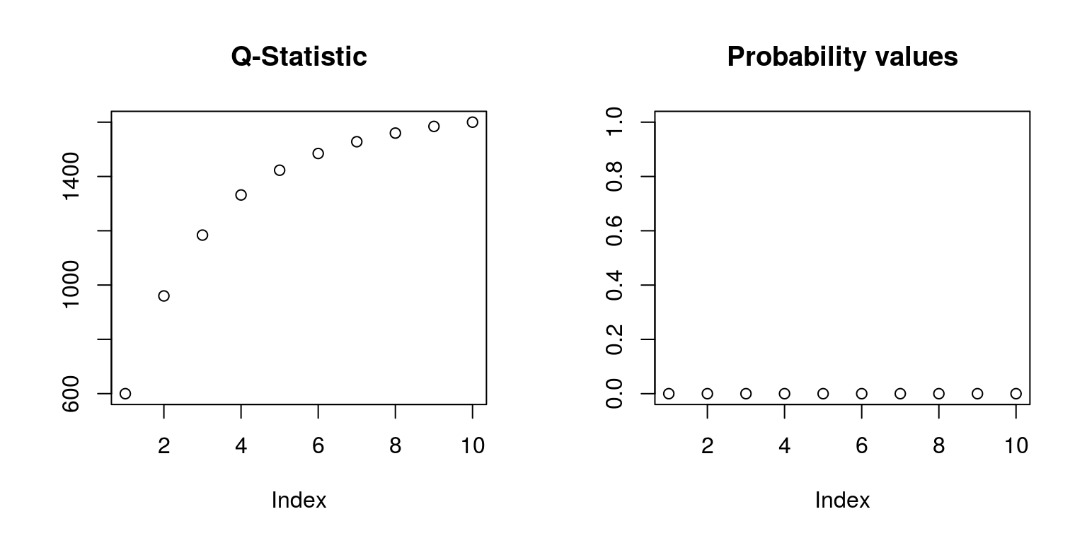
par(op) # close plot areaThese p-value values suggest that there is significant autocorrelation in this time series process. To speed up the above computation you should vectorize your code and use the apply functions in R, which would be important when dealing with routines or statistics that take a long time to compute.
We can now fit a model to this process with the aid of an AR(1) specification and look at the results that are stored in the arma10 object that we have created.
arma10 <- arima(x, order = c(1, 0, 0), include.mean = FALSE)  # uses ARIMA(p,d,q) specification
arma10
##
## Call:
## arima(x = x, order = c(1, 0, 0), include.mean = FALSE)
##
## Coefficients:
## ar1
## 0.7783
## s.e. 0.0199
##
## sigma^2 estimated as 1.006: log likelihood = -1422.49, aic = 2848.98To take a look at what the residuals look like we plot the residuals that are stored in the arma10 object.
par(mfrow = c(1, 1))
plot(arma10$residuals)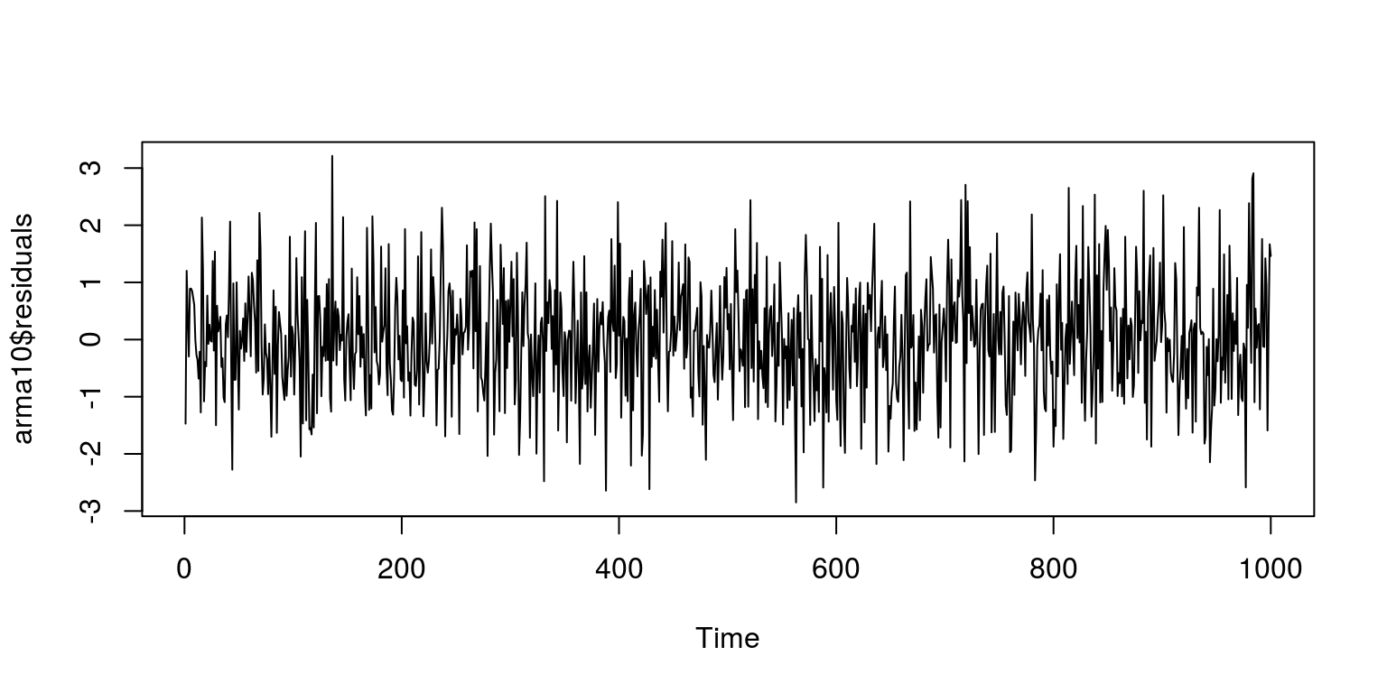
Now lets take a look at the ACF and PACF for the residuals
ac(arma10$residuals, max.lag = 18)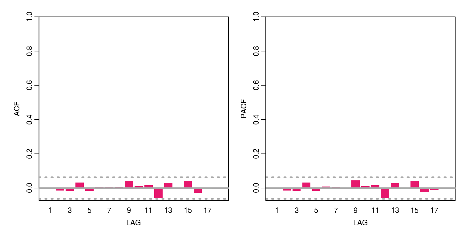
There would appear to be no serial correlation in the residual.
3 Simulated moving average process
Now lets generate a MA(1) process and store the values in an object that we call y.
y <- arima.sim(model = list(ma = 0.7), n = 1000)As is always the case, the first thing that we do is visually inspect the data.
par(mfrow = c(1, 1))
plot.ts(y)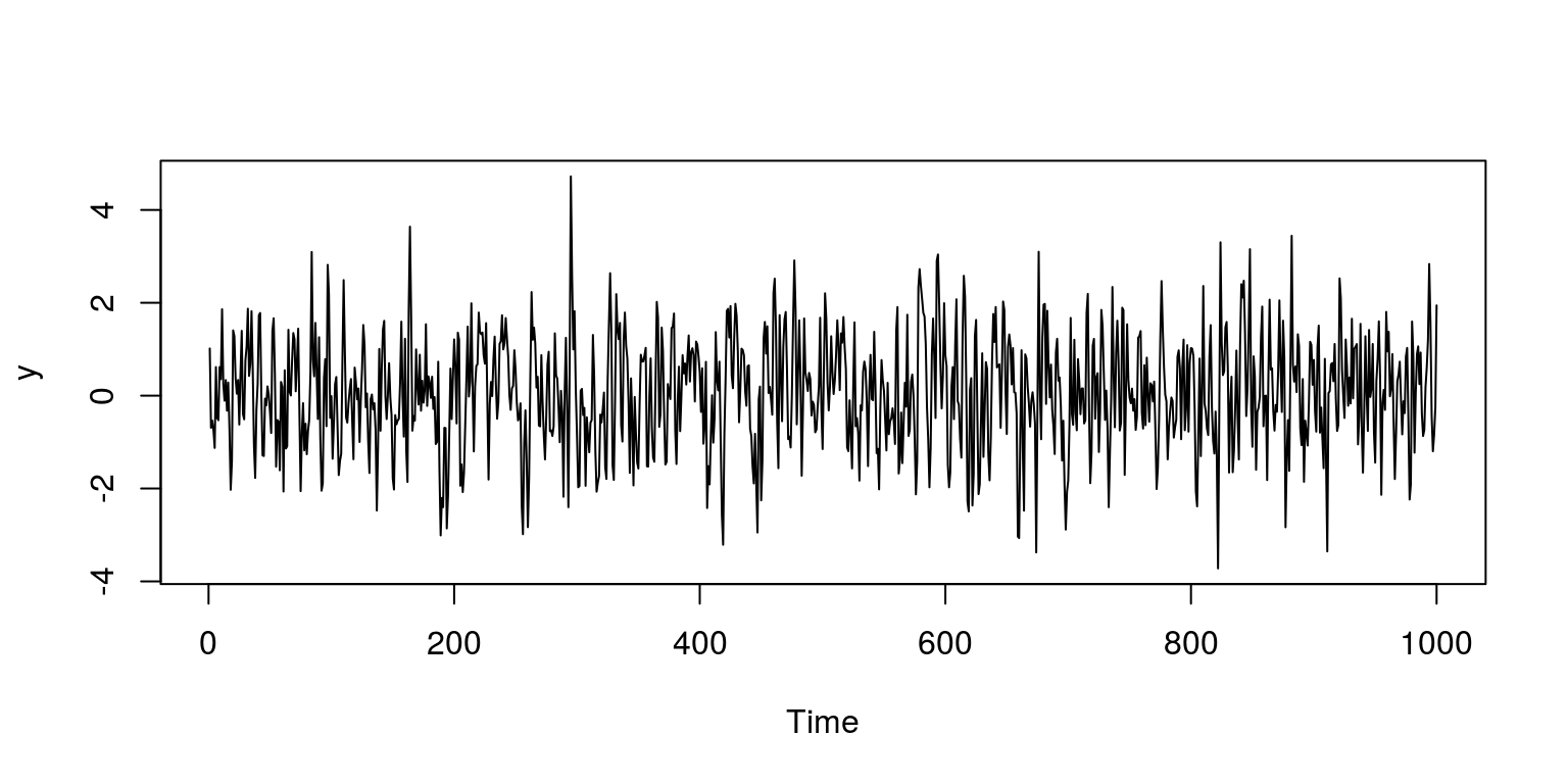
We can then consider the ACF and PACF for this variable.
ac(y, max.lag = 18)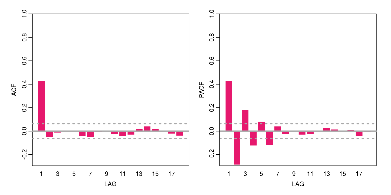
To fit a first-order moving average model to the data, where the estimation results are stored in the object arma01 we execute the commands:
arma01 <- arima(y, order = c(0, 0, 1))  # uses ARIMA(p,d,q) with constant
arma01
##
## Call:
## arima(x = y, order = c(0, 0, 1))
##
## Coefficients:
## ma1 intercept
## 0.6929 0.0634
## s.e. 0.0237 0.0534
##
## sigma^2 estimated as 0.9962: log likelihood = -1417.38, aic = 2840.75To inspect the residuals we execute the following commands and would note that they take on features of white noise.
par(mfrow = c(1, 1))
plot(arma01$residuals)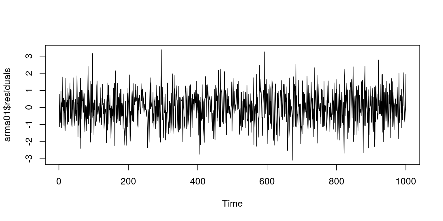
ac(arma01$residuals, max.lag = 18)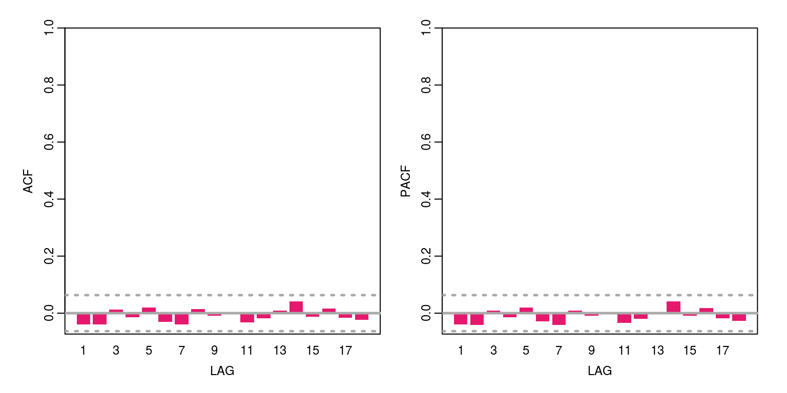
4 Simulated ARMA process
As noted in the lectures, the values of autocorrelation and partial autocorrelation functions for an ARMA process is equivalent to some form of weighted sum of these functions for the individual autoregressive and moving average components. This is displayed below, where we firstly simulate the autoregressive and moving average components before we provide the results of the ARMA process.
x <- arima.sim(model = list(ar = 0.4), n = 200)  # AR(1) process
ac(x, max.lag = 20)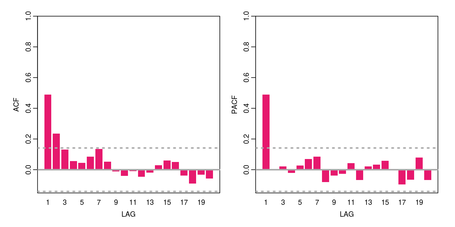
x <- arima.sim(model = list(ma = 0.5), n = 200)  # MA(1) process
ac(x, max.lag = 20)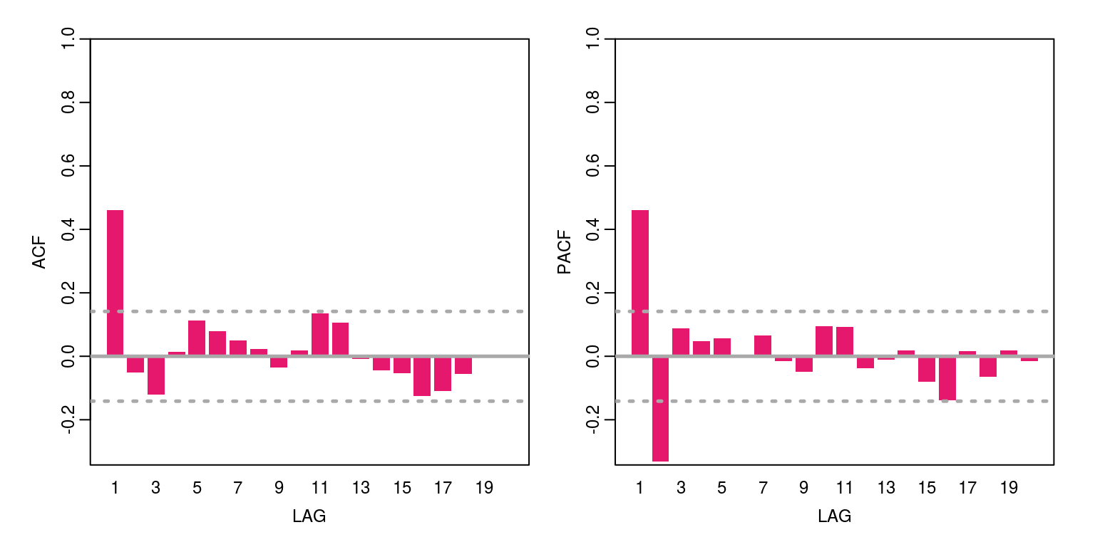
x <- arima.sim(model = list(ar = 0.4, ma = 0.5), n = 200)  ## ARMA(1,1)
ac(x, max.lag = 20)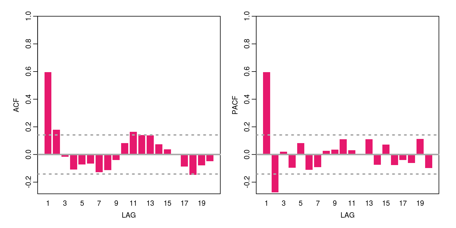
In the following exercise we will simulate an ARMA(2,1) process and try to see whether we can identify it without any prior knowledge. To identify the process we will make use of the ACF & PACF as well as the information criteria.
z <- arima.sim(model = list(ar = c(0.6, -0.2), ma = c(0.4)),
    n = 200)
ac(z, max.lag = 18)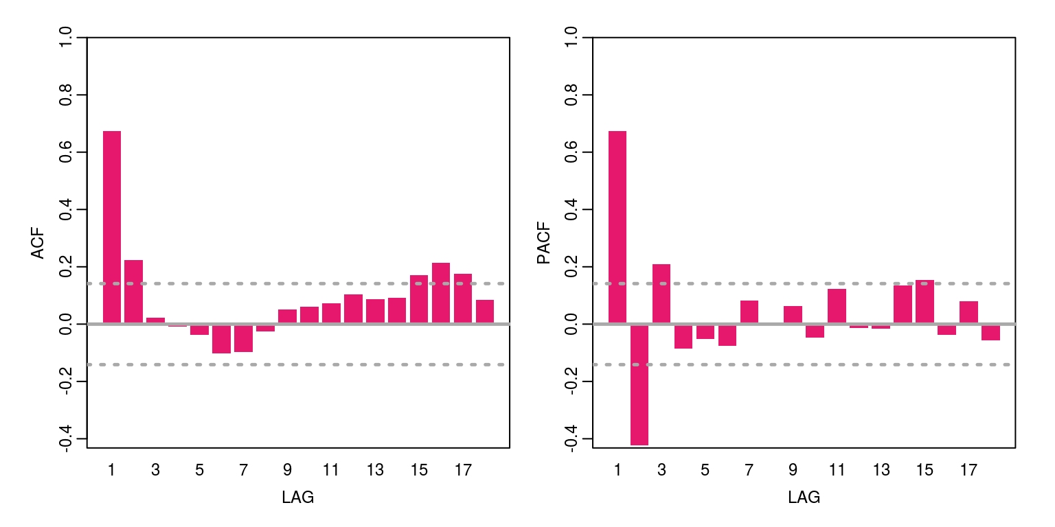
The results from the ACF & PACF would suggest that we are at most dealing with an ARMA(3,2). To estimate all models that may have an order that is equal to or less than order we could proceed as follows, before storing the AIC value in the object arma.res.
arma.res <- rep(0, 16)
arma.res[1] <- arima(z, order = c(3, 0, 2))$aic  # fit arma(3,2) and save aic value
arma.res[2] <- arima(z, order = c(2, 0, 2))$aic
arma.res[3] <- arima(z, order = c(2, 0, 1))$aic
arma.res[4] <- arima(z, order = c(1, 0, 2))$aic
arma.res[5] <- arima(z, order = c(1, 0, 1))$aic
arma.res[6] <- arima(z, order = c(3, 0, 0))$aic
arma.res[7] <- arima(z, order = c(2, 0, 0))$aic
arma.res[8] <- arima(z, order = c(0, 0, 2))$aic
arma.res[9] <- arima(z, order = c(3, 0, 2), include.mean = FALSE)$aic
arma.res[10] <- arima(z, order = c(2, 0, 2), include.mean = FALSE)$aic
arma.res[11] <- arima(z, order = c(2, 0, 1), include.mean = FALSE)$aic
arma.res[12] <- arima(z, order = c(1, 0, 2), include.mean = FALSE)$aic
arma.res[13] <- arima(z, order = c(1, 0, 1), include.mean = FALSE)$aic
arma.res[14] <- arima(z, order = c(3, 0, 0), include.mean = FALSE)$aic
arma.res[15] <- arima(z, order = c(2, 0, 0), include.mean = FALSE)$aic
arma.res[16] <- arima(z, order = c(0, 0, 2), include.mean = FALSE)$aic
To find the model that has the lowest value for the AIC statistic we could execute the code:
which(arma.res == min(arma.res))## [1] 13This would suggest that ARMA(1,1) would provide a suitable fit for the model, which is perfect, but lets have a look at the dianostics. Hence, we re-estimate the model, store all the results and consider whether there is serial correlation in the residuals.
arma11 <- arima(z, order = c(1, 0, 1), include.mean = FALSE)
ac(arma11$residuals, max.lag = 20)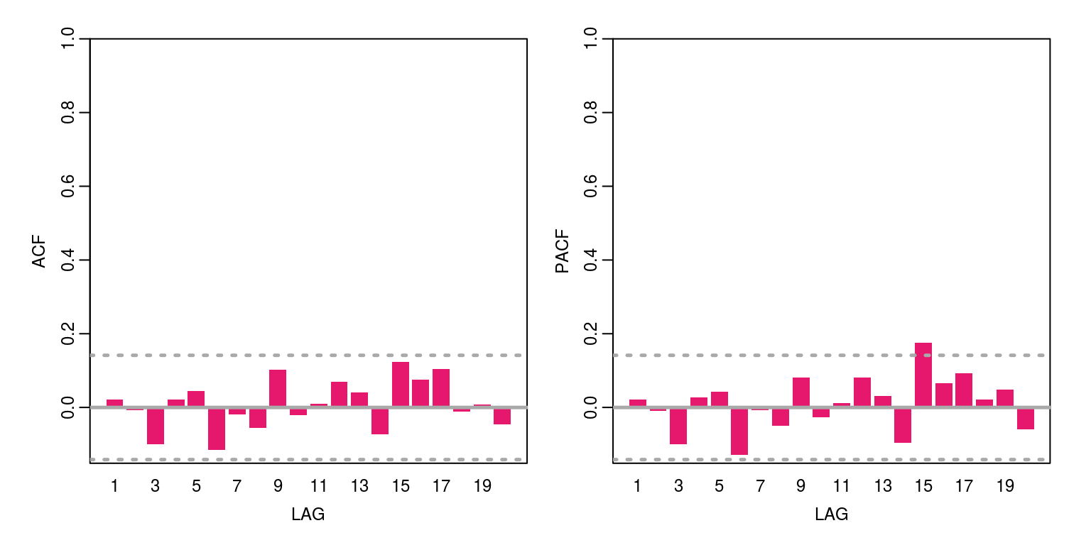
Q.stat <- rep(NA, 10)  # vector of ten observations
Q.prob <- rep(NA, 10)

for (i in 4:10) {
    Q.stat[i] <- Box.test(arma11$residuals, lag = i, type = "Ljung-Box",
        fitdf = 3)$statistic
    Q.prob[i] <- Box.test(arma11$residuals, lag = i, type = "Ljung-Box",
        fitdf = 3)$p.value
}

op <- par(mfrow = c(1, 2))
plot(Q.stat, ylab = "", main = "Q-Statistic")
plot(Q.prob, ylab = "", ylim = c(0, 1), main = "Probability values")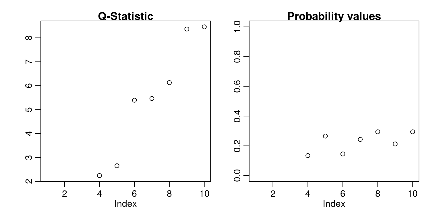
par(op)This would appear to provide suitable results.
5 Structural breaks
To test for structural breaks we can make use of the strucchange package that may be found on the cran repository. Before you install these new packages, you may wish to clear the workspace environment and closing down all graphics by running the commands:
rm(list = ls())
graphics.off()
To install this package from cran we could use the Packages tab on and click on install or one could enter the command: install.packages('strucchange'). Thereafter, we make use of the library command to access the routines in this package:
library(strucchange)To generate AR(1) and white noise processes with 100 observations, where we make use of the same seed value, we execute the following commands:
set.seed(123)  # setting the seed so we all get the same results
x1 <- arima.sim(model = list(ar = 0.9), n = 100)  # simulate 100 obs for AR(1)
x2 <- rnorm(100)  # simulate 100 obs for white noise process
To join these two time series variables, we make use of the concatenate command that would leave us with a structural break after observation 100.
y <- c((10 + x1), x2)
plot.ts(y)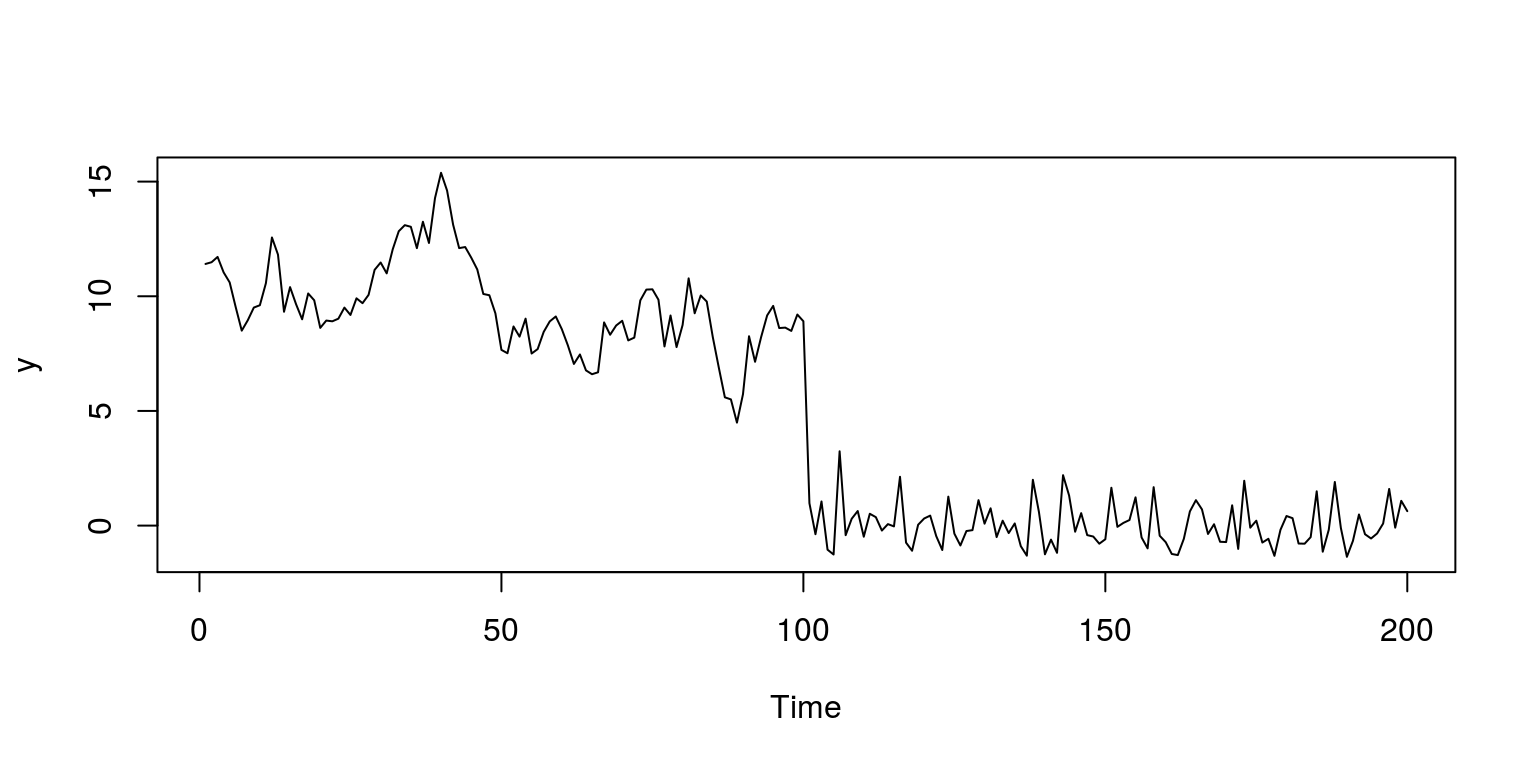
The underlying model that we are going to use to describe this process is an AR(1), however, before we are able to execute these tests, we need to organise our variables in a small data-frame. To arrange the variable of interest and a lagged variant of this variable in a data.frame we make use of the following commands:
dat <- data.frame(cbind(y[-1], y[-(length(y))]))
colnames(dat) <- c("ylag0", "ylag1")
Thereafter, we can make use of the QLR statistic that takes the form of an F-test to detect a possible structural break.
fs <- Fstats(ylag0 ~ ylag1, data = dat)
breakpoints(fs)  # where the breakpoint is
##
## Optimal 2-segment partition:
##
## Call:
## breakpoints.Fstats(obj = fs)
##
## Breakpoints at observation number:
## 99
##
## Corresponding to breakdates:
## 0.4924623sctest(fs, type = "supF") # the significance of this breakpoint##
## supF test
##
## data: fs
## sup.F = 184.43, p-value < 2.2e-16plot(fs)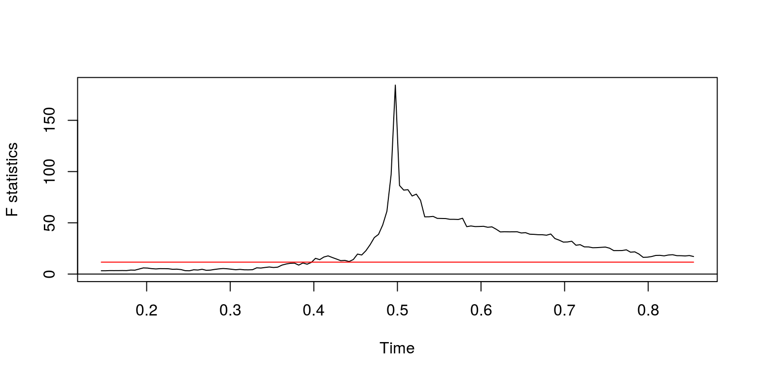
These results suggest that there is a structural break that originates at observation 99 (after we lost an observation due to taking lags). In addition, we note that the p-value would suggest that this break is statstically significant and the plot confirms this, as the F-statistic breaks through the confidence interval.
As an alternative we can make use of the CUSUM test statistic that may be executed with the commands:
cusum <- efp(ylag0 ~ ylag1, type = "OLS-CUSUM", data = dat)
plot(cusum)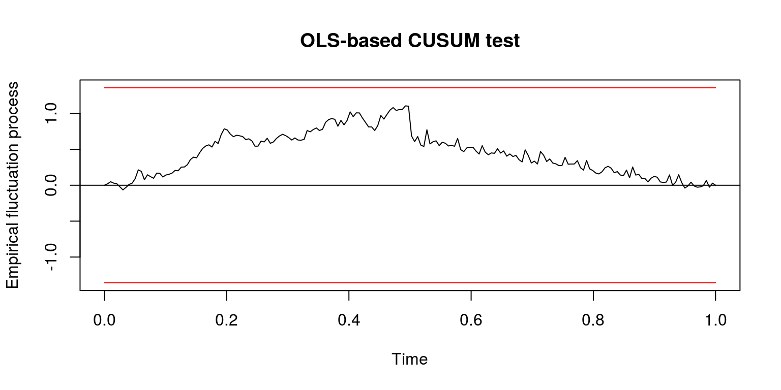
Note that in this case the test does not suggest that there is a structural break as the value of the coefficient is not subject to any sudden change. This should not be terribly surprising as the addition of white noise would not add any additional information to the part of the regression model that is to be explained, which would not influence the value of the coefficient by a great deal.
6 Univariate models for real data
6.1 South African gross domestic product
Before we work through the next part of this tutorial we will clear the workspace environment again and close all the figures that we have plotted.
rm(list = ls())
graphics.off()
In this tutorial we would like to make use of the tsm and strucchange packages so we run the commands:
library(tsm)
library(strucchange)
All the data for this tut has been preloaded in the tsm package. It includes the most recent measures of South African Real Gross Domestic Product that is published by the South African Reserve Bank, which has the code KBP6006D. Hence, to retrieve the data from the package and create the object for the series as dat, we execute the following commands:
dat <- sarb_quarter$KBP6006D
dat.tmp <- diff(log(na.omit(dat)) * 100, lag = 1)
head(dat)
## [1] 565040 574255 584836 590609 594892 592293gdp <- ts(dat.tmp, start = c(1960, 2), frequency = 4)Note that the object dat.tmp is the quarter-on-quarter growth rate for this variable, after all na’s have been removed. Since the first observation in this time series is 1960q2, we can create a time series object for this variable that is labelled gdp. To make sure that these calculations and extractions have been performed correctly, we can plot this data
plot.ts(gdp)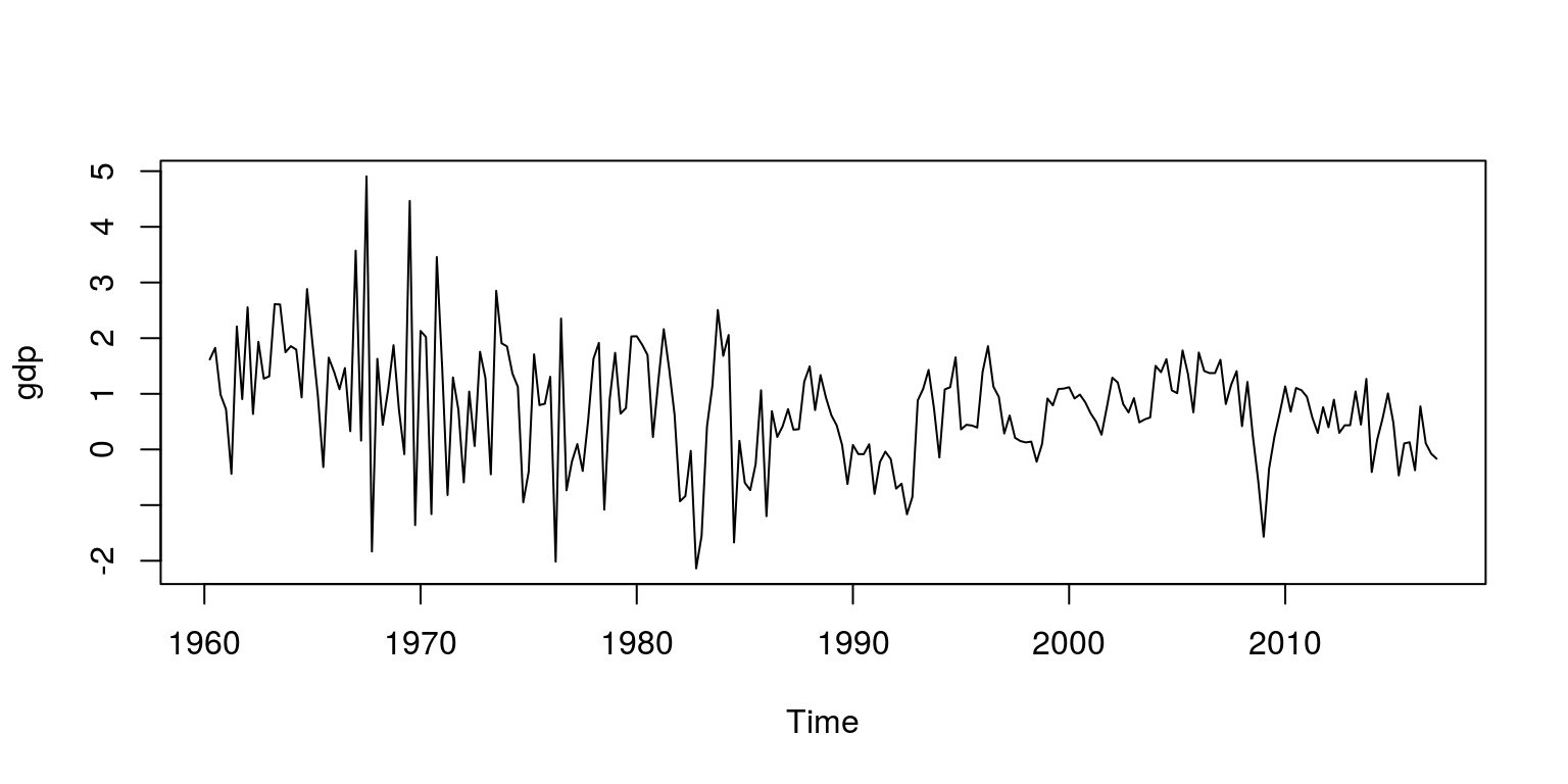
If we are of the opinion that this seems reasonable, we can proceed by checking for structural breaks. In this instance, we once again make use of an AR(1) model, so we create a dataframe for the variables:
dat.gdp <- cbind(gdp, lag(gdp, k = -1))
colnames(dat.gdp) <- c("ylag0", "ylag1")
dat.gdp <- window(dat.gdp, start = c(1960, 3))
Thereafter, we can generate QLR statistic with the commands:
fs <- Fstats(ylag0 ~ ylag1, data = dat.gdp)
breakpoints(fs)
##
## Optimal 2-segment partition:
##
## Call:
## breakpoints.Fstats(obj = fs)
##
## Breakpoints at observation number:
## 42
##
## Corresponding to breakdates:
## 0.1806167sctest(fs, type = "supF")##
## supF test
##
## data: fs
## sup.F = 73.391, p-value = 3.461e-15plot(fs)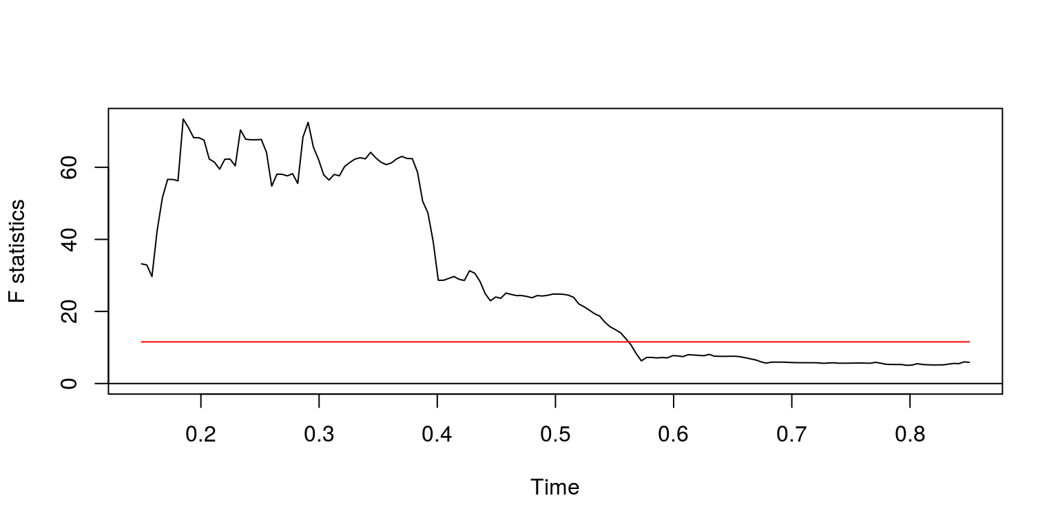
These results suggest that there may be a couple of breakpoints. The first structural break would appear to arise during the early 1970’s, so we exclude the first part of the time series with the command:
dat.gdp1 <- window(dat.gdp, start = c(1972, 1))To consider whether or not the remaining time series contains a structural break we generate the QLR statistic once again.
fs <- Fstats(ylag0 ~ ylag1, data = dat.gdp1)
breakpoints(fs)
##
## Optimal 2-segment partition:
##
## Call:
## breakpoints.Fstats(obj = fs)
##
## Breakpoints at observation number:
## 32
##
## Corresponding to breakdates:
## 0.1712707sctest(fs, type = "supF")##
## supF test
##
## data: fs
## sup.F = 23.192, p-value = 0.0002651plot(fs)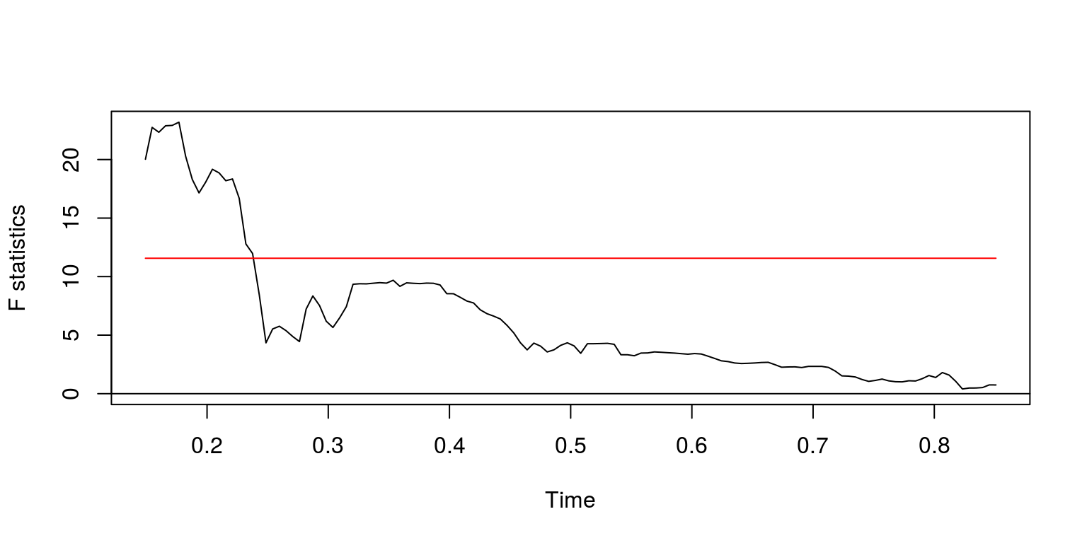
As this suggests that there is another structural break around 1908, we consider the test statistics for the remaining information
dat.gdp2 <- window(dat.gdp, start = c(1980, 4))
fs <- Fstats(ylag0 ~ ylag1, data = dat.gdp2)
breakpoints(fs)
##
## Optimal 2-segment partition:
##
## Call:
## breakpoints.Fstats(obj = fs)
##
## Breakpoints at observation number:
## 49
##
## Corresponding to breakdates:
## 0.3287671sctest(fs, type = "supF")##
## supF test
##
## data: fs
## sup.F = 5.9882, p-value = 0.421plot(fs)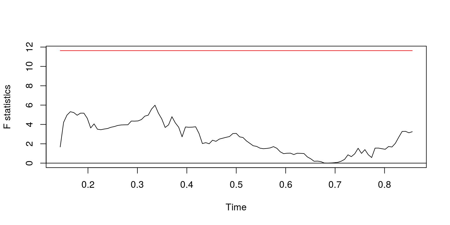
This would appear to be satisfactory. We will then label this subsample y and can consider the degree of autocorrelation.
y <- window(gdp, start = c(1981, 1))
ac(as.numeric(y))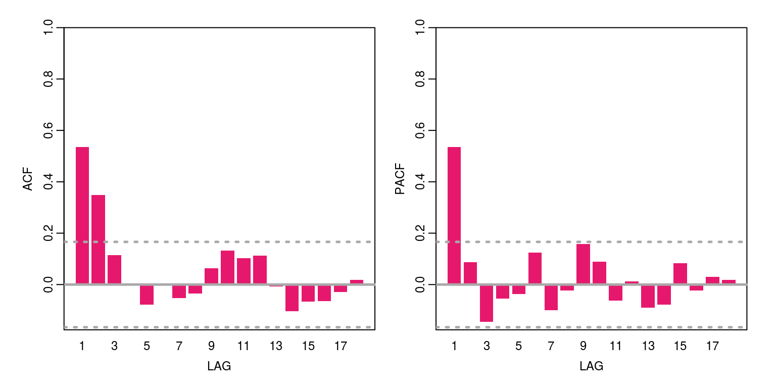
This variable has a bit of persistence and does not appear to be nonstationary. The maximum order of this variable is an AR(1), MA(2), or some combination of the two. We can then check the information criteria for a number of candidate models by constructing the following vector for the statistics:
arma.res <- rep(0, 5)
arma.res[1] <- arima(y, order = c(1, 0, 2))$aic
arma.res[2] <- arima(y, order = c(1, 0, 1))$aic
arma.res[3] <- arima(y, order = c(1, 0, 0))$aic
arma.res[4] <- arima(y, order = c(0, 0, 2))$aic
arma.res[5] <- arima(y, order = c(0, 0, 1))$aic
To find the model with the smallest AIC value we can then execute the command:
which(arma.res == min(arma.res))## [1] 1These results suggest that the smallest value is provided by ARMA(1,2). With this in mind we estimate the parameter values for this model structure.
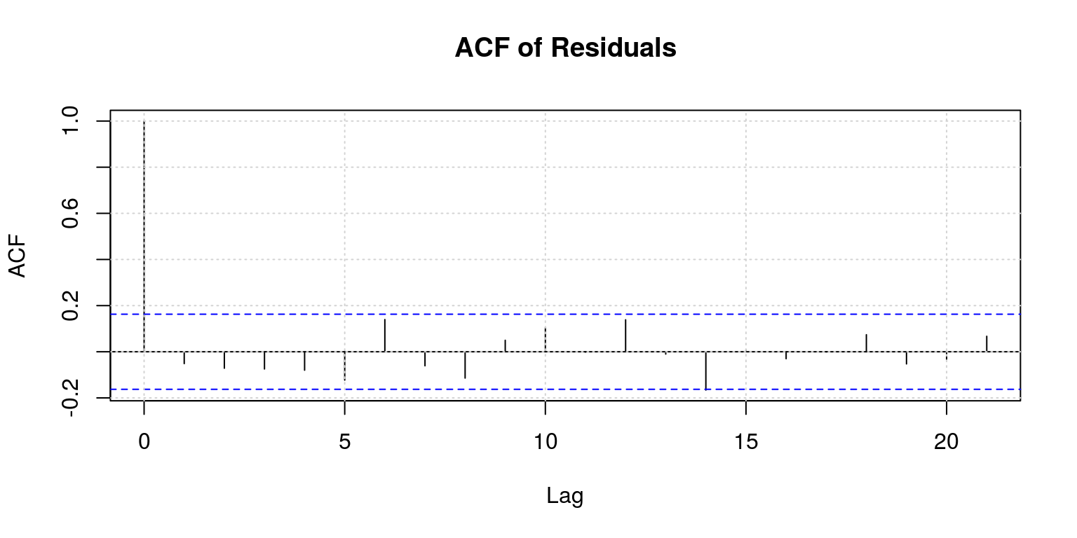
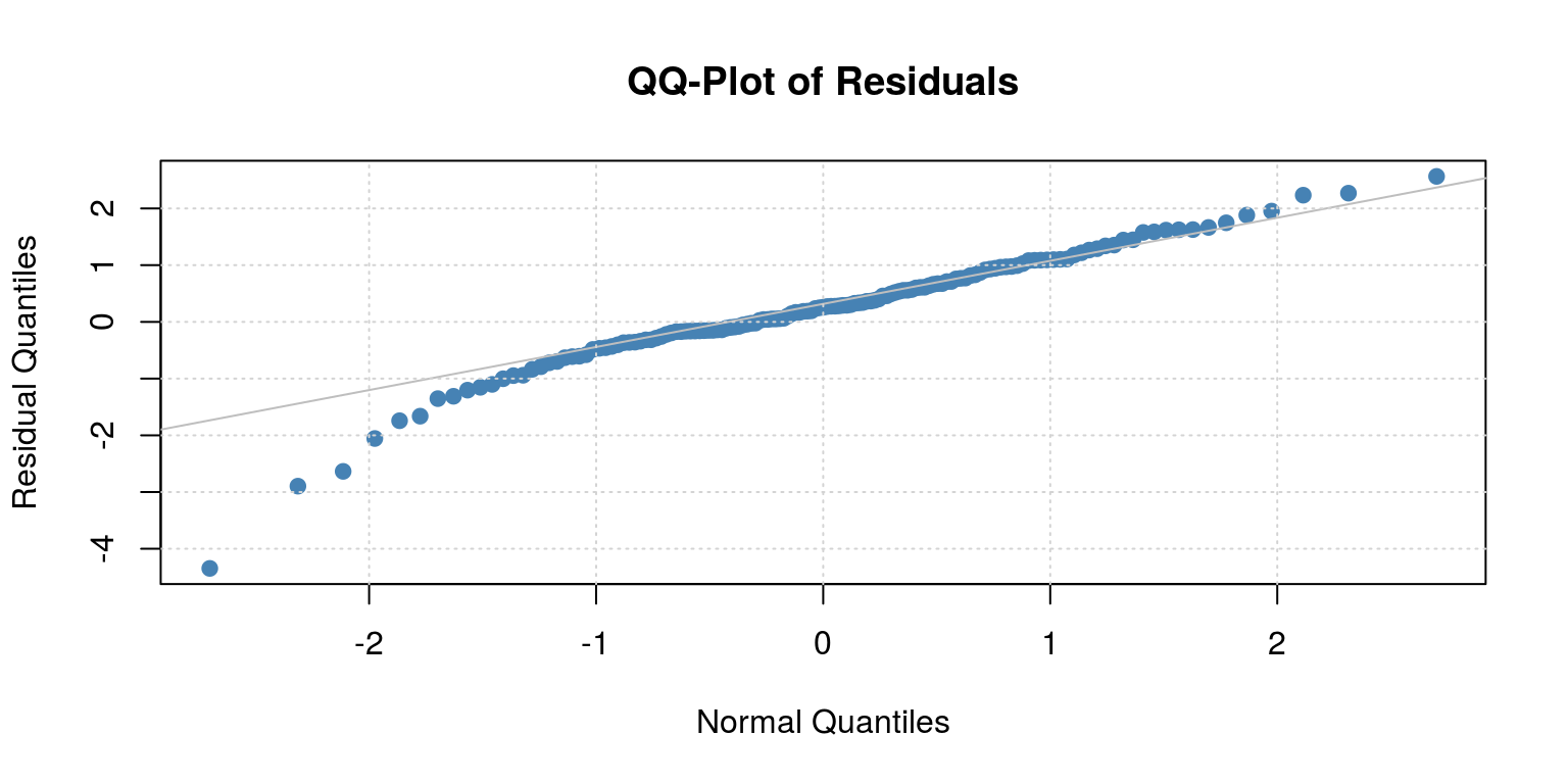
arma <- arima(y, order = c(1, 0, 2))Thereafter, we look at the residuals for the model to determine if there is any serial correlation.
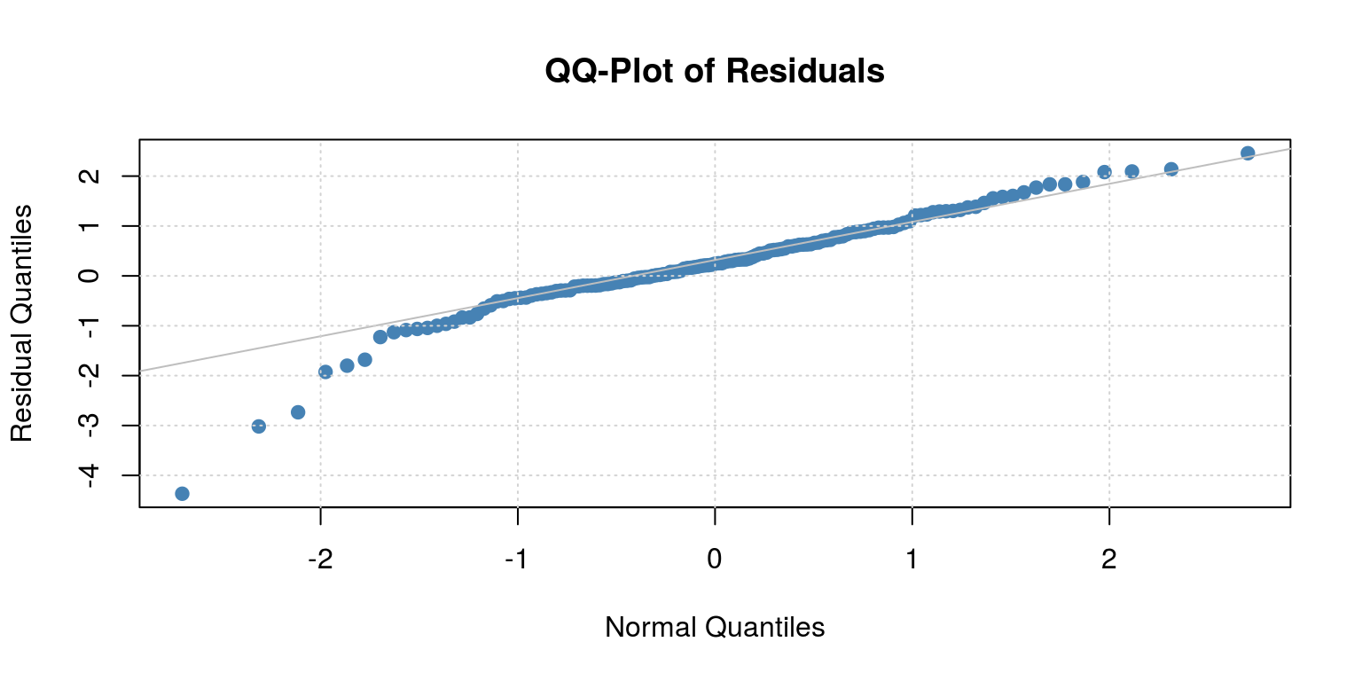
par(mfrow = c(1, 1))
plot(arma$residuals)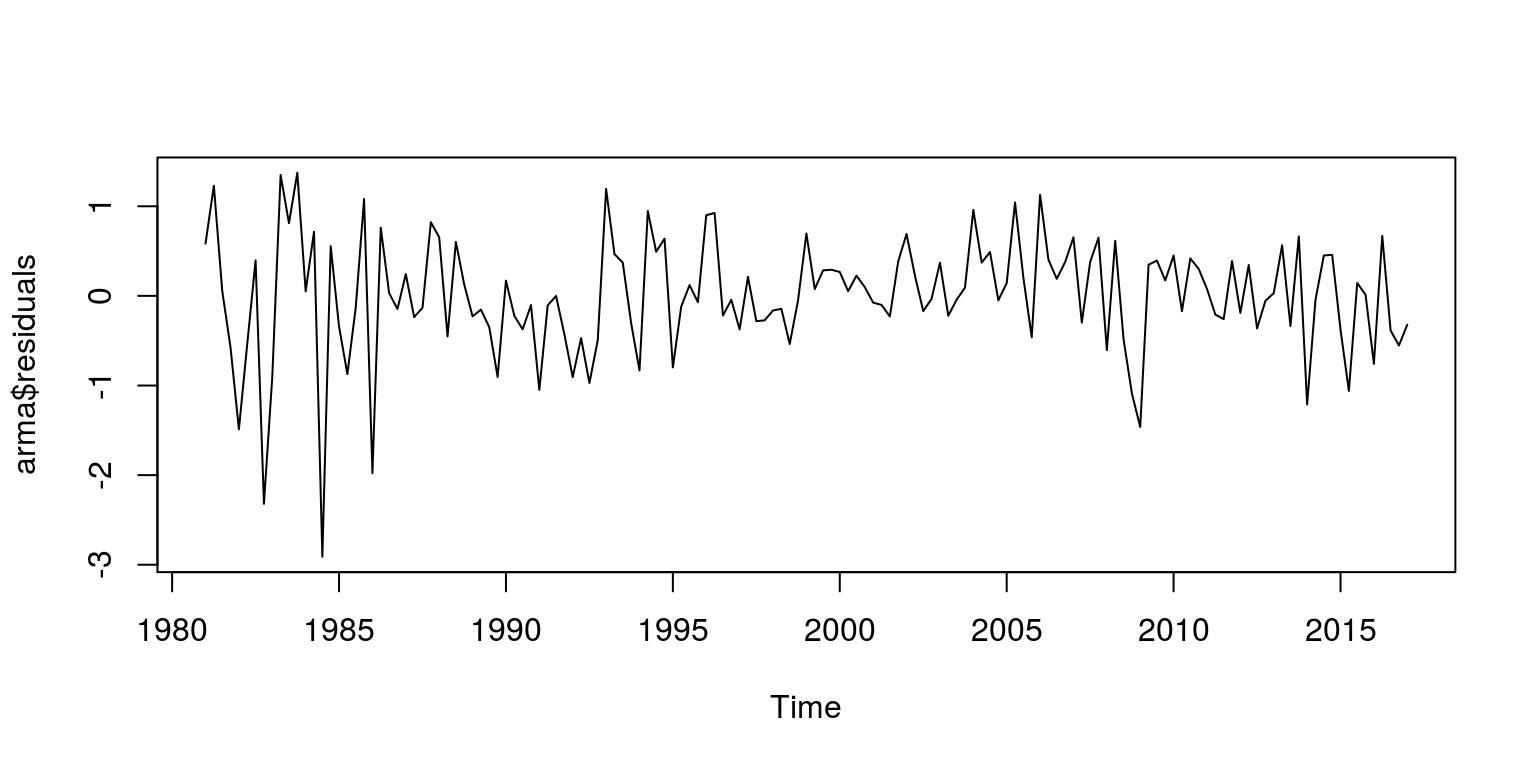
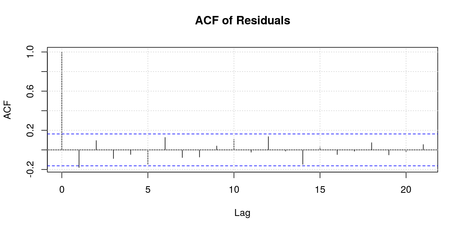
ac(arma$residuals)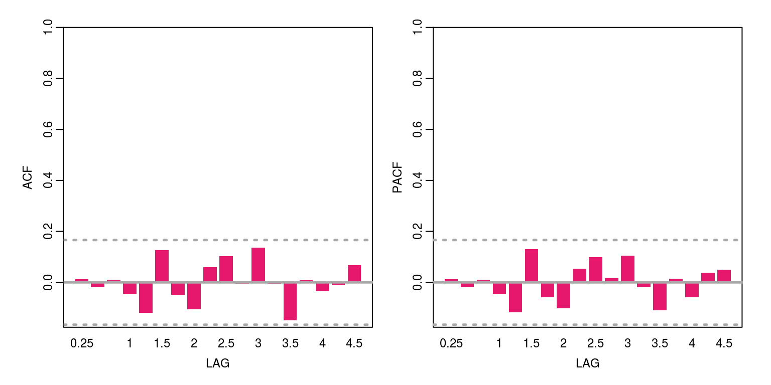
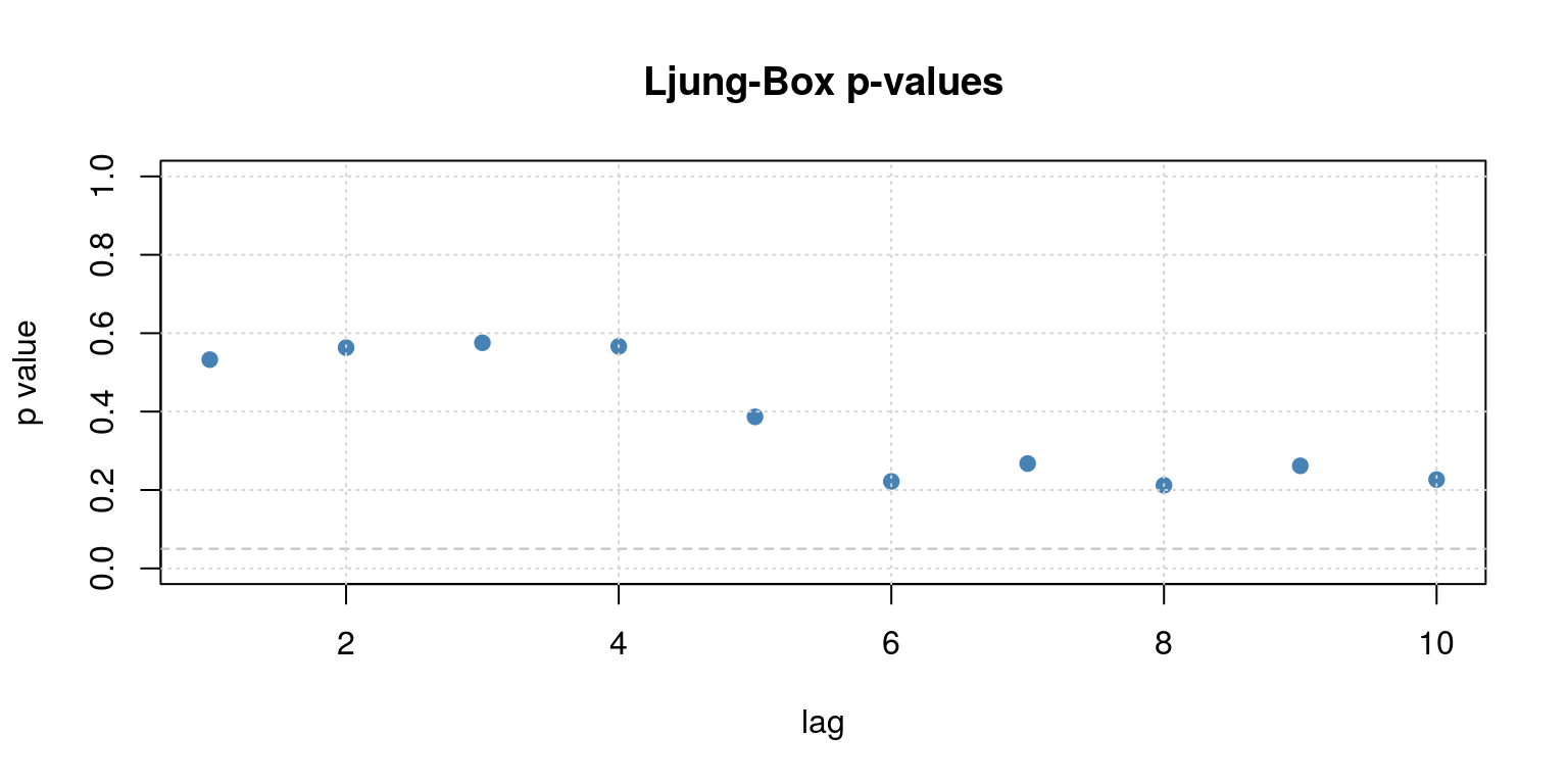
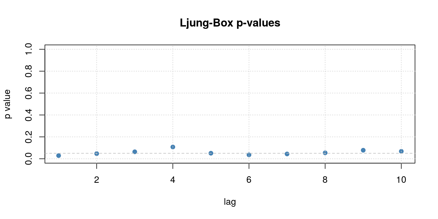
These results suggests that there is no remaining serial correlation, but we could also take a look at the Q-statistics to confirm this.
Q.stat <- rep(NA, 12)
Q.prob <- rep(NA, 12)

for (i in 6:12) {
    Q.stat[i] <- Box.test(arma$residuals, lag = i, type = "Ljung-Box",
        fitdf = 2)$statistic
    Q.prob[i] <- Box.test(arma$residuals, lag = i, type = "Ljung-Box",
        fitdf = 2)$p.value
}

op <- par(mfrow = c(1, 2))
plot(Q.stat, ylab = "", main = "Q-Statistic")
plot(Q.prob, ylab = "", ylim = c(0, 1), main = "Probability values")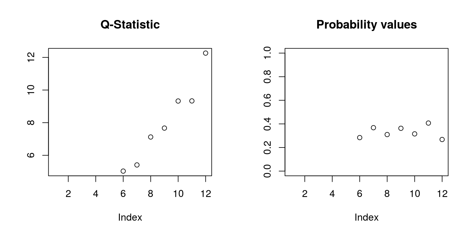
par(op)There certainly don’t appear to be too many problems here. However, given the level of persistence that is suggested by the autocorrelation function, the model may be over-parameterised. Recall that all the results from the model estimation are stored in the object arma and we could derive the t-statistics from the standard errors. However, there is another package, which is named fArma that displays these results in a more convenient manner. To dowload this package we could click on the install button that is located on the Packages tab, or we could run the command install.packages('fArma') in the Console. Once the package is installed, we use the library command to access the routines. Thereafter, we estimate the model with the armaFit command.
library(fArma)
fit1 <- armaFit(~arma(1, 2), data = y, include.mean = FALSE)
summary(fit1)
##
## Title:
## ARIMA Modelling
##
## Call:
## armaFit(formula = ~arma(1, 2), data = y, include.mean = FALSE)
##
## Model:
## ARIMA(1,0,2) with method: CSS-ML
##
## Coefficient(s):
## ar1 ma1 ma2
## 0.6817 -0.1041 0.1697
##
## Residuals:
## Min 1Q Median 3Q Max
## -2.9969 -0.1345 0.1774 0.5720 1.7684
##
## Moments:
## Skewness Kurtosis
## -0.931 3.157
##
## Coefficient(s):
## Estimate Std. Error t value Pr(>|t|)
## ar1 0.6817 0.1206 5.654 1.57e-08 ***
## ma1 -0.1041 0.1351 -0.771 0.441
## ma2 0.1697 0.1262 1.345 0.179
## ---
## Signif. codes:
## 0 '***' 0.001 '**' 0.01 '*' 0.05 '.' 0.1 ' ' 1
##
## sigma^2 estimated as: 0.4755
## log likelihood: -152.2
## AIC Criterion: 312.41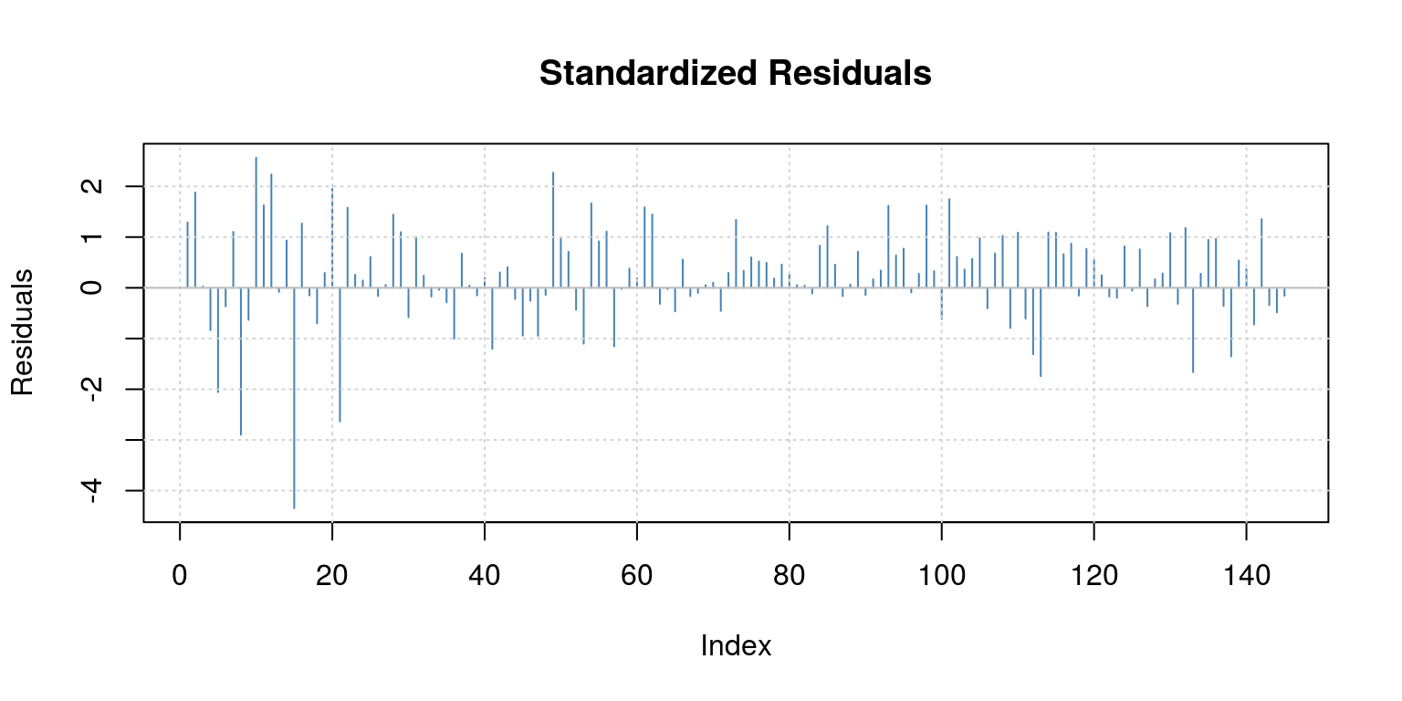
##
## Description:
##  Sun Aug  5 23:39:52 2018 by user:
Note that the MA(1) and MA(2) parameters do not appear to be significant, so we should drop them and just estimate an AR(1) model.
fit2 <- armaFit(~arma(1, 0), data = y, include.mean = FALSE)
summary(fit2)
##
## Title:
## ARIMA Modelling
##
## Call:
## armaFit(formula = ~arma(1, 0), data = y, include.mean = FALSE)
##
## Model:
## ARIMA(1,0,0) with method: CSS-ML
##
## Coefficient(s):
## ar1
## 0.6787
##
## Residuals:
## Min 1Q Median 3Q Max
## -3.0669 -0.1380 0.1714 0.5859 1.7269
##
## Moments:
## Skewness Kurtosis
## -0.9986 3.4459
##
## Coefficient(s):
## Estimate Std. Error t value Pr(>|t|)
## ar1 0.67872 0.06068 11.18 <2e-16 ***
## ---
## Signif. codes:
## 0 '***' 0.001 '**' 0.01 '*' 0.05 '.' 0.1 ' ' 1
##
## sigma^2 estimated as: 0.4932
## log likelihood: -154.8
## AIC Criterion: 313.61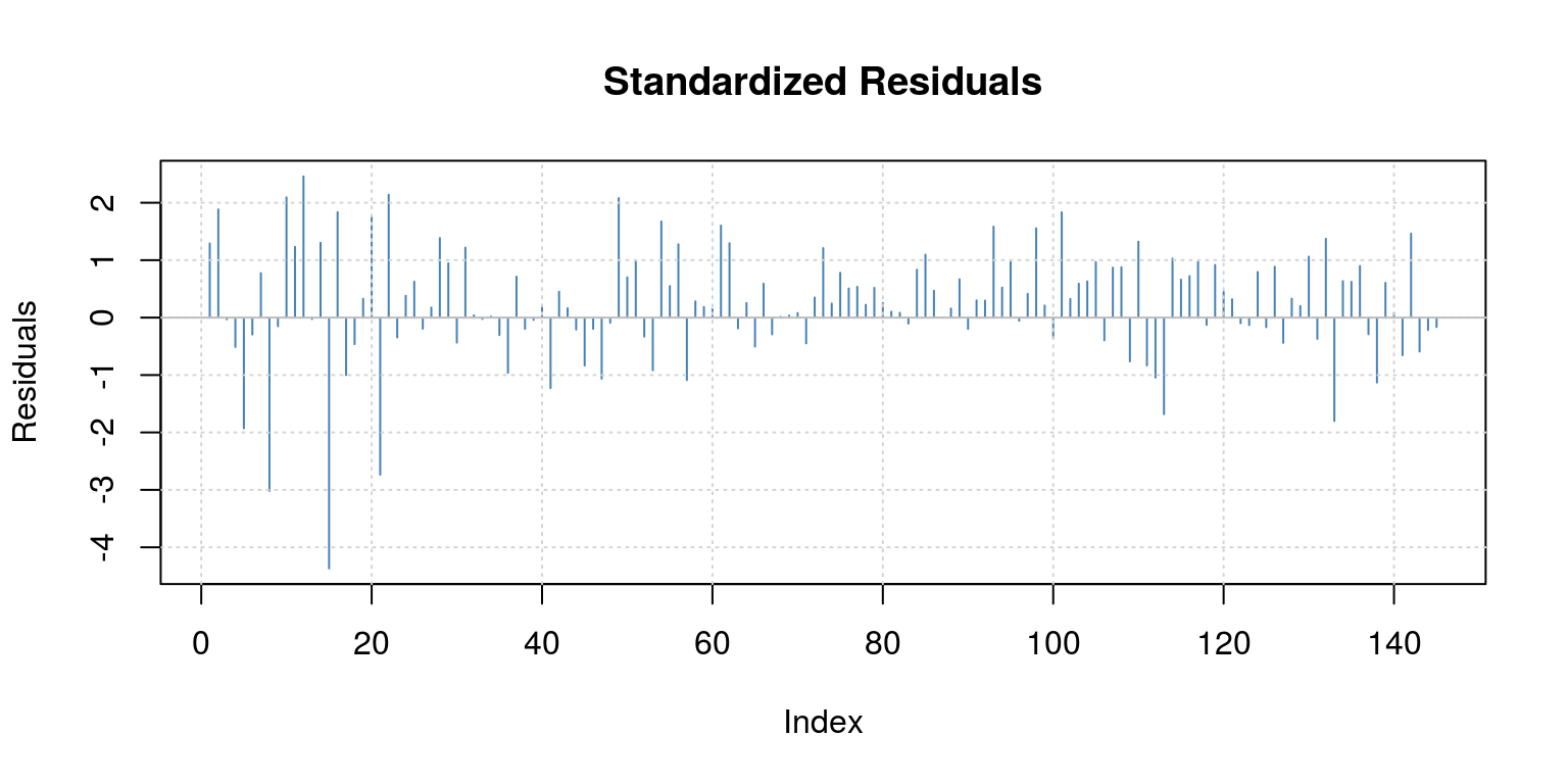
##
## Description:
##  Sun Aug  5 23:39:52 2018 by user:
Another useful package is the forecast package, which you would know how to install by now. After you provide yourself with access to the routines in the package, you can utilise the auto.arima command, which allows you to specify the maximum number of autoregressive and moveing average lags. Thereafter, you can decide which information criteria should be used to select the final model and everything will be done for you.
library(forecast)
auto.mod <- auto.arima(y, max.p = 2, max.q = 2, start.p = 0,
    start.q = 0, stationary = TRUE, seasonal = FALSE, allowdrift = FALSE,
    ic = "aic")

auto.mod  # AR(2) with intercept
## Series: y
## ARIMA(1,0,0) with non-zero mean
##
## Coefficients:
## ar1 mean
## 0.5375 0.5295
## s.e. 0.0699 0.1197
##
## sigma^2 estimated as 0.4578: log likelihood=-148.26
## AIC=302.53 AICc=302.7 BIC=311.46As the name suggests, this package has a number of useful forecasting routines, which is the subject of next weeks lecture. For example, to generate a forecast for the last 4 years of data, we remove the out-of-sample data from that which is going to be used for the insample estimation. In this case, we can compare the out-of-sample results for the ARIMA(1,2) with the AR(1) model.
y.sub <- window(y, start = c(1981, 1), end = c(2012, 1),
    frequency = 4)
arma10 <- arima(y.sub, order = c(1, 0, 0))
arma12 <- arima(y.sub, order = c(1, 0, 2))
To forecast foreward we can use the predict command, as follows:
arma10.pred <- predict(arma10, n.ahead = 16)
arma12.pred <- predict(arma12, n.ahead = 16)
To plot these results we would use the plot.ts and lines commands that is used for displaying the results on the same set of axes.
plot.ts(y)
lines(arma10.pred$pred, col = "blue", lty = 2)
lines(arma12.pred$pred, col = "green", lty = 2)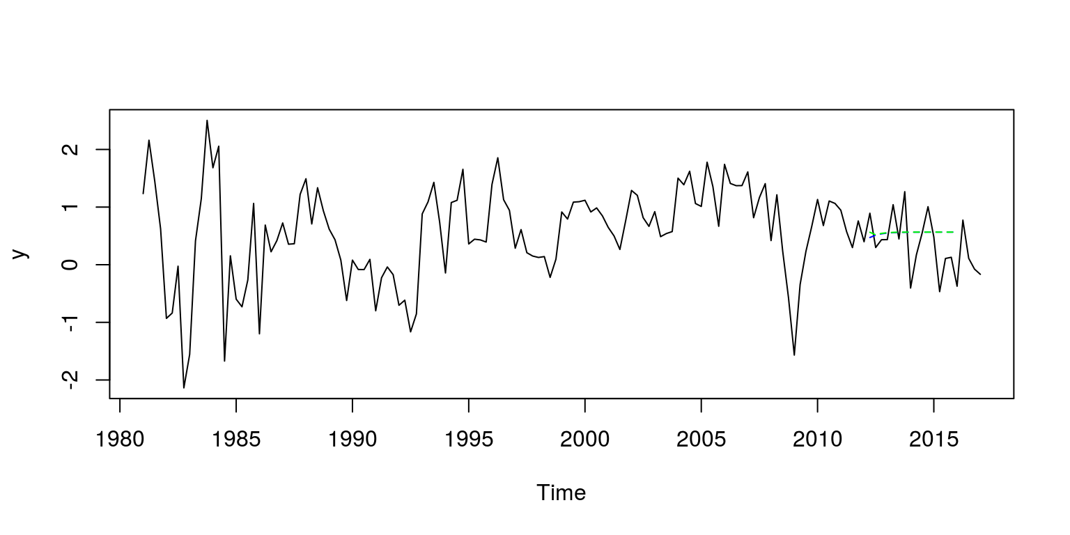
Or alternatively, if we just want to focus on the last few years of data:
y.act <- window(y, start = c(2011, 1), end = c(2016, 1))
fore.11 <- c(rep(NA, 5), arma10.pred$pred[1:16])
fore.32 <- c(rep(NA, 5), arma12.pred$pred[1:16])
fore.res <- cbind(as.numeric(y.act), fore.11, fore.32)

plot.ts(fore.res, plot.type = "single", col = c("black",
    "blue", "green"))
legend("bottomleft", legend = c("actual", "arma11", "arma32"),
    lty = c(1, 1, 1), col = c("black", "blue", "green"),
    bty = "n")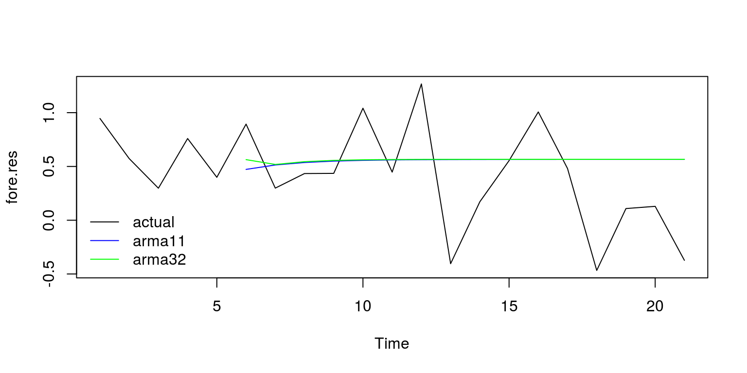
Unfortunately, these forecasting results look fairly poor.
6.2 South African consumer price index
Once again, we will start off this part of the tutorial by clearing the workspace environment and closing all the plots.
rm(list = ls())
graphics.off()
Once again we are going to make use of the tsm and strucchange packages so we run the commands:
library(tsm)
library(strucchange)
To access the CPI data in the tsm package, we would want to extract the series KBP7170N that is published by the South African Reserve Bank on a monthly basis. To get data that is slightly more current, you would go to the Statistics South Africa website. This series starts in January 2002. Hence, we can execute the following commands:
dat <- sarb_month$KBP7170N
cpi <- ts(na.omit(dat), start = c(2002, 1), frequency = 12)
To calculate month-on-month and year-on-year inflation rates, we perform the following transformations and plot the data to make sure that it looks reasonable.
inf.mom <- diff(cpi, lag = 1)/cpi[-length(cpi)]
inf.yoy <- diff(cpi, lag = 12)/cpi[-1 * (length(cpi) - 11):length(cpi)]
plot.ts(inf.yoy)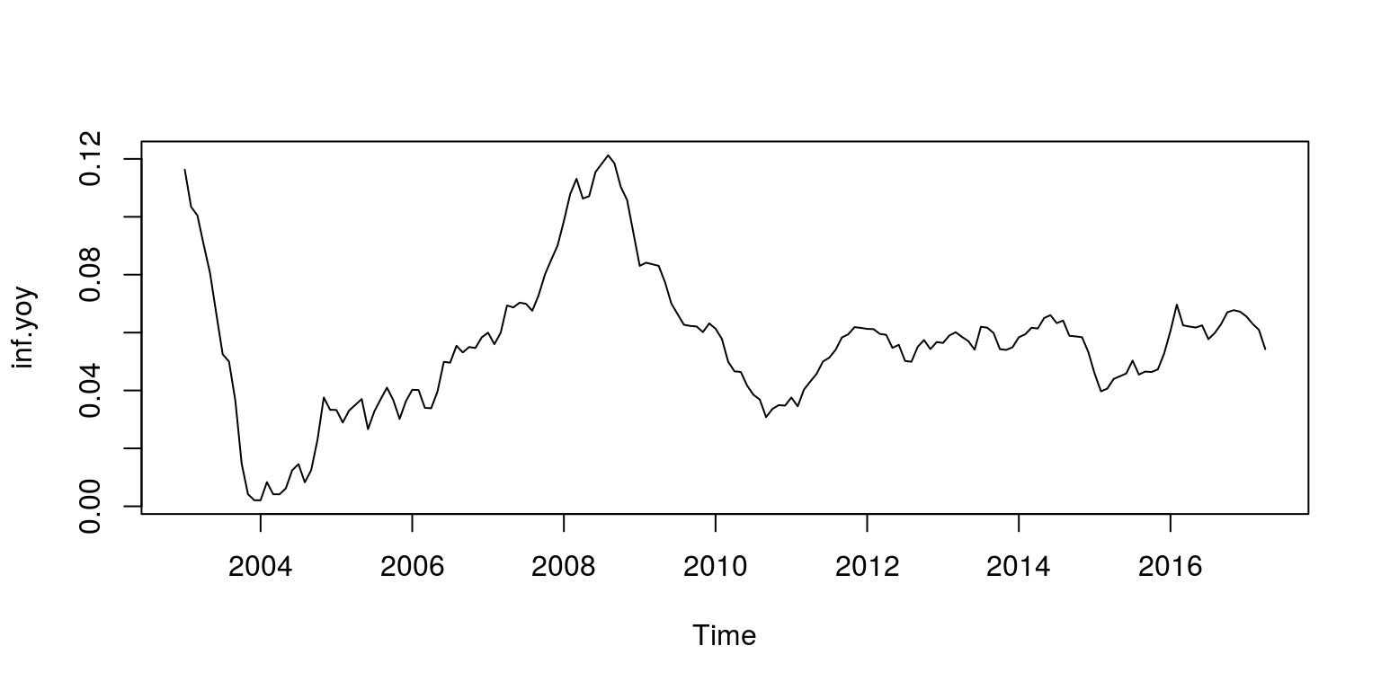
We can then proceed to check for structural breaks. In this instance, we once again make use of an AR(1) model, so we create a database for the variables:
dat.inf <- cbind(inf.yoy, lag(inf.yoy, k = -1))
colnames(dat.inf) <- c("ylag0", "ylag1")
Thereafter, we can generate QLR statistic with the commands:
fs <- Fstats(ylag0 ~ ylag1, data = dat.inf)
breakpoints(fs)
##
## Optimal 2-segment partition:
##
## Call:
## breakpoints.Fstats(obj = fs)
##
## Breakpoints at observation number:
## 25
##
## Corresponding to breakdates:
## 0.1403509sctest(fs, type = "supF")##
## supF test
##
## data: fs
## sup.F = 31.201, p-value = 5.847e-06plot(fs)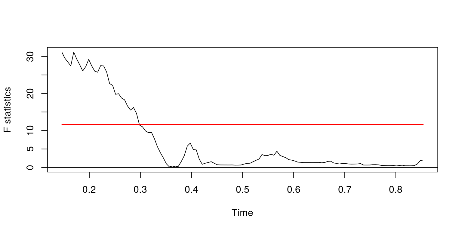
In addition, we can look at the results of the CUSUM statistic.
cusum <- efp(ylag0 ~ ylag1, type = "OLS-CUSUM", data = dat.inf)
plot(cusum)  # there certainly appears to be some change in the first part of the sample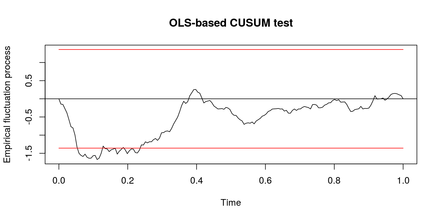
These results suggest that there could be a breakpoint immediately prior to 2005M2, so let’s take a subset of data for the susequent periods of time.
y <- window(inf.yoy, start = c(2005, 2))We can now take a look at the persistence in the data, by plotting the autocorrelation function. Note that the first autocorrelation coefficient is around 0.97, which suggests that this could be a random-walk process. As such we should test for a unit root by using ADF (or similar) test, but as we are only going to cover this topic in a later lecture, we are going to proceed as if the process is stationary.
ac(as.numeric(y))
If we allow for a maximum order for an AR(2) and/or an MA(4) - although the moving average component could be of a higher order, we can then check the information criteria for a number of candidate models by constructing the following vector for the statistics:
arma.res <- rep(0, 8)
arma.res[1] <- arima(y, order = c(2, 0, 4))$aic
arma.res[2] <- arima(y, order = c(2, 0, 3))$aic
arma.res[3] <- arima(y, order = c(2, 0, 2))$aic
arma.res[4] <- arima(y, order = c(2, 0, 1))$aic
arma.res[5] <- arima(y, order = c(2, 0, 0))$aic
arma.res[6] <- arima(y, order = c(1, 0, 2))$aic
arma.res[7] <- arima(y, order = c(1, 0, 1))$aic
arma.res[8] <- arima(y, order = c(1, 0, 0))$aic
To find the model with the smallest AIC value we can then execute the command:
which(arma.res == min(arma.res))## [1] 5These results suggest that the smallest value is provided by ARMA(2,0). With this in mind we estimate the parameter values for this model structure.
arma <- arima(y, order = c(2, 0, 0))Thereafter, we look at the residuals for the model to determine if there is any serial correlation.
par(mfrow = c(1, 1))
plot(arma$residuals)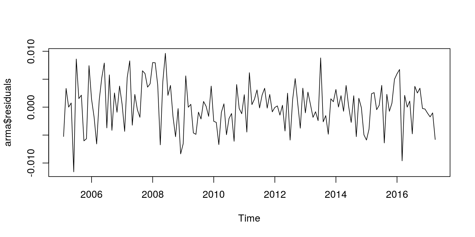
ac(arma$residuals)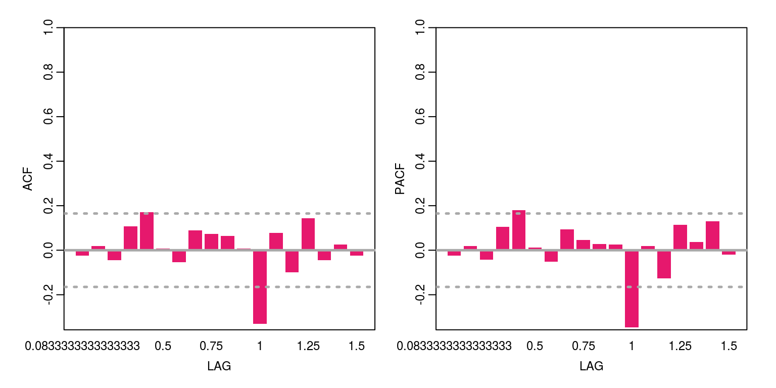
These results suggests that there is still some autocorrelation year-on-year. To estimate a arma model with seasonal components, we need to install the astsa package, using the install button on the Packages tab or the command, install.packages('astsa'). In this case, we will fit two variants of the model, where the sarima(x,2,0,0,0,1,1,12) command will fit a SARIMA(2,0,0)*(0,1,1)_{12} model.
library(astsa)

sarima1 <- sarima(y, 2, 0, 0, 0, 0, 0, 12)  # sarima(x,p,d,q,P,D,Q,S) where sarima(x,2,0,0,0,1,1,12) will fit SARIMA(2,0,0)*(0,1,1)_{12}
## initial value -3.939766
## iter 2 value -4.393484
## iter 3 value -5.245578
## iter 4 value -5.317399
## iter 5 value -5.431991
## iter 6 value -5.482457
## iter 7 value -5.507663
## iter 8 value -5.510206
## iter 9 value -5.510214
## iter 10 value -5.510219
## iter 11 value -5.510289
## iter 12 value -5.510324
## iter 13 value -5.510325
## iter 13 value -5.510325
## iter 13 value -5.510325
## final value -5.510325
## converged
## initial value -5.493801
## iter 2 value -5.494032
## iter 3 value -5.494922
## iter 4 value -5.495098
## iter 5 value -5.495204
## iter 6 value -5.495313
## iter 7 value -5.495545
## iter 8 value -5.495843
## iter 9 value -5.495905
## iter 10 value -5.495968
## iter 11 value -5.496045
## iter 12 value -5.496089
## iter 13 value -5.496102
## iter 14 value -5.496103
## iter 14 value -5.496103
## iter 14 value -5.496103
## final value -5.496103
## converged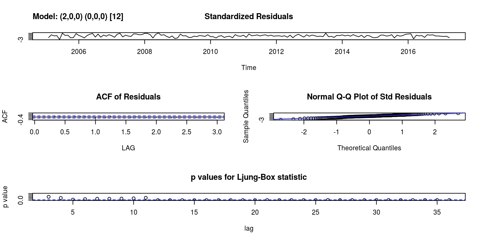
names(sarima1)## [1] "fit" "degrees_of_freedom"
## [3] "ttable" "AIC"
## [5] "AICc" "BIC"names(sarima1$fit)## [1] "coef" "sigma2" "var.coef" "mask"
## [5] "loglik" "aic" "arma" "residuals"
## [9] "call" "series" "code" "n.cond"
## [13] "nobs" "model"par(mfrow = c(1, 1))
plot(sarima1$fit$residuals)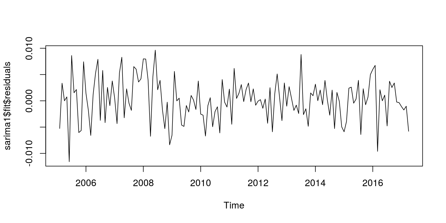
ac(as.numeric(sarima1$fit$residuals))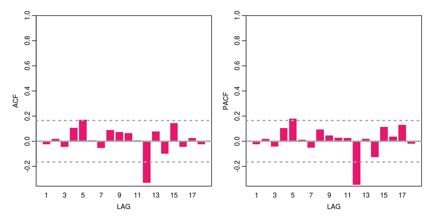
sarima2 <- sarima(y, 2, 0, 1, 1, 0, 0, 12) # sarima(x,p,d,q,P,D,Q,S) where sarima(x,2,1,0,0,1,1,12) will fit SARIMA(2,1,0)*(0,1,1)_{12}## initial value -3.964652
## iter 2 value -4.511039
## iter 3 value -5.062536
## iter 4 value -5.214318
## iter 5 value -5.439984
## iter 6 value -5.515829
## iter 7 value -5.612132
## iter 8 value -5.614171
## iter 9 value -5.614431
## iter 10 value -5.617334
## iter 11 value -5.622557
## iter 12 value -5.631673
## iter 13 value -5.633969
## iter 14 value -5.635143
## iter 15 value -5.635894
## iter 16 value -5.638322
## iter 17 value -5.640541
## iter 18 value -5.642155
## iter 19 value -5.642269
## iter 20 value -5.642300
## iter 21 value -5.642306
## iter 22 value -5.642347
## iter 23 value -5.642365
## iter 24 value -5.642365
## iter 25 value -5.642366
## iter 26 value -5.642367
## iter 27 value -5.642368
## iter 28 value -5.642369
## iter 29 value -5.642370
## iter 30 value -5.642370
## iter 30 value -5.642370
## iter 30 value -5.642370
## final value -5.642370
## converged
## initial value -5.561956
## iter 2 value -5.564498
## iter 3 value -5.566343
## iter 4 value -5.568918
## iter 5 value -5.570030
## iter 6 value -5.571417
## iter 7 value -5.573604
## iter 8 value -5.574429
## iter 9 value -5.577166
## iter 10 value -5.579282
## iter 11 value -5.584058
## iter 12 value -5.585552
## iter 13 value -5.585927
## iter 14 value -5.586857
## iter 15 value -5.588030
## iter 16 value -5.590170
## iter 17 value -5.592098
## iter 18 value -5.593931
## iter 19 value -5.594933
## iter 20 value -5.595478
## iter 21 value -5.595661
## iter 22 value -5.595957
## iter 23 value -5.596126
## iter 24 value -5.596163
## iter 25 value -5.596196
## iter 26 value -5.596209
## iter 27 value -5.596226
## iter 28 value -5.596247
## iter 29 value -5.596263
## iter 30 value -5.596273
## iter 31 value -5.596278
## iter 32 value -5.596281
## iter 33 value -5.596282
## iter 34 value -5.596283
## iter 34 value -5.596283
## final value -5.596283
## converged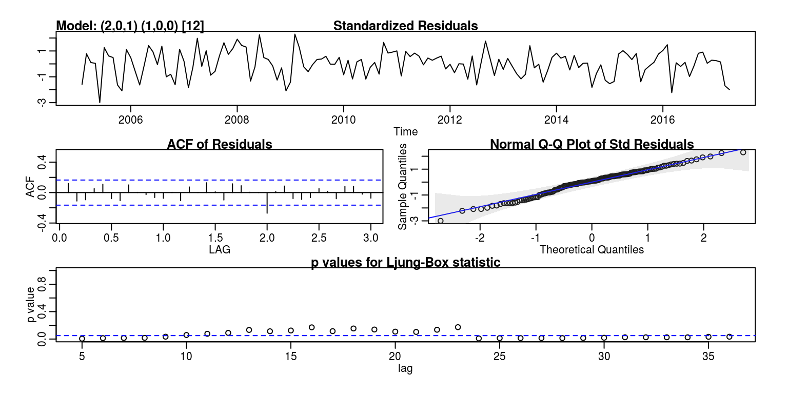
ac(as.numeric(sarima2$fit$residuals))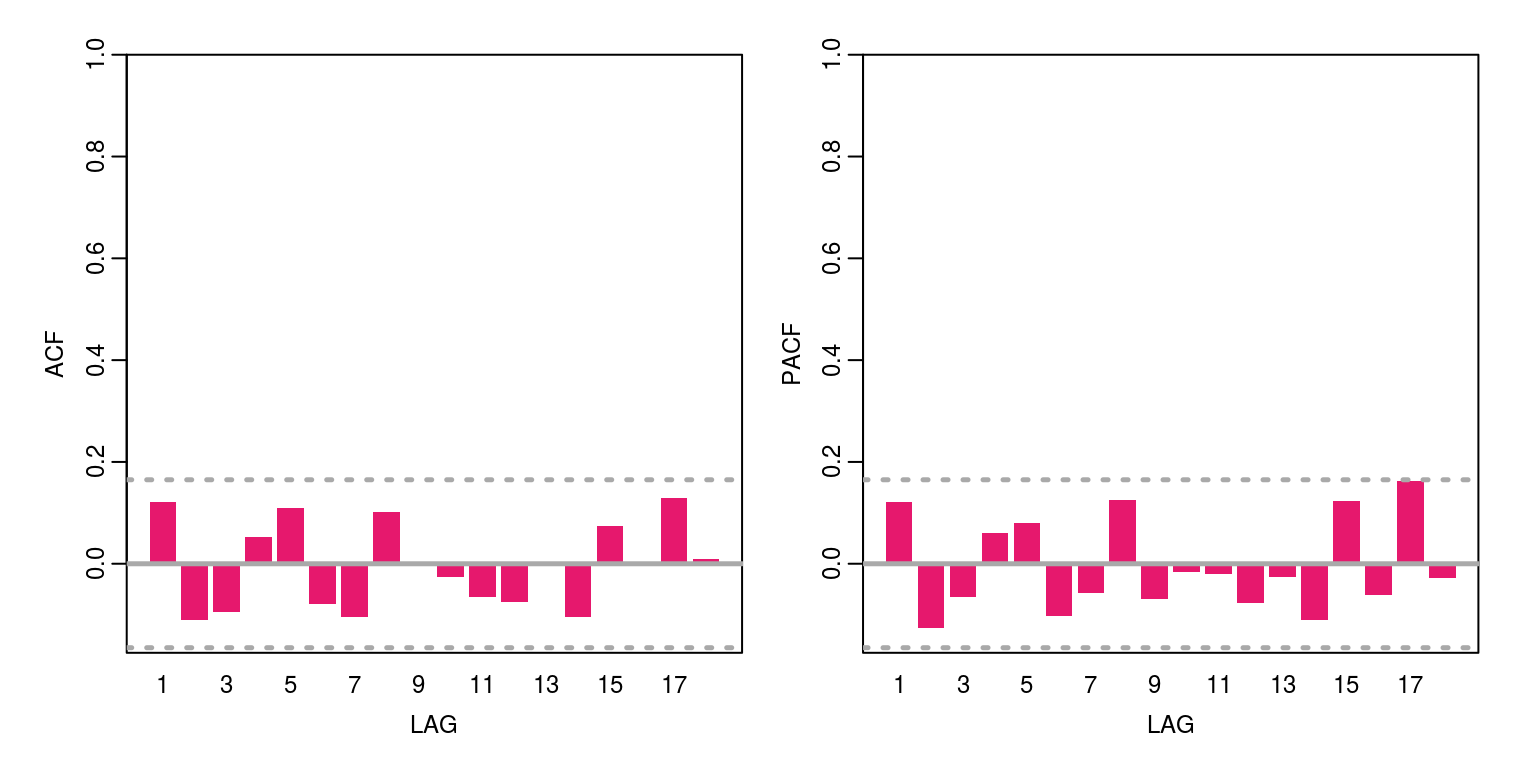
In the second of these models we note that the seasonal information has been effectively captured by the monthly seasonal component. Once again we can generate a forecast for this model with the aid of the following commands:
library(fArma)
y.sub <- window(y, end = c(2016, 12))

par(mfrow = c(1, 1))
forcast1 <- sarima.for(y.sub, 2, 0, 1, 1, 0, 0, 12, n.ahead = 4)
lines(y, col = "green", lty = 1)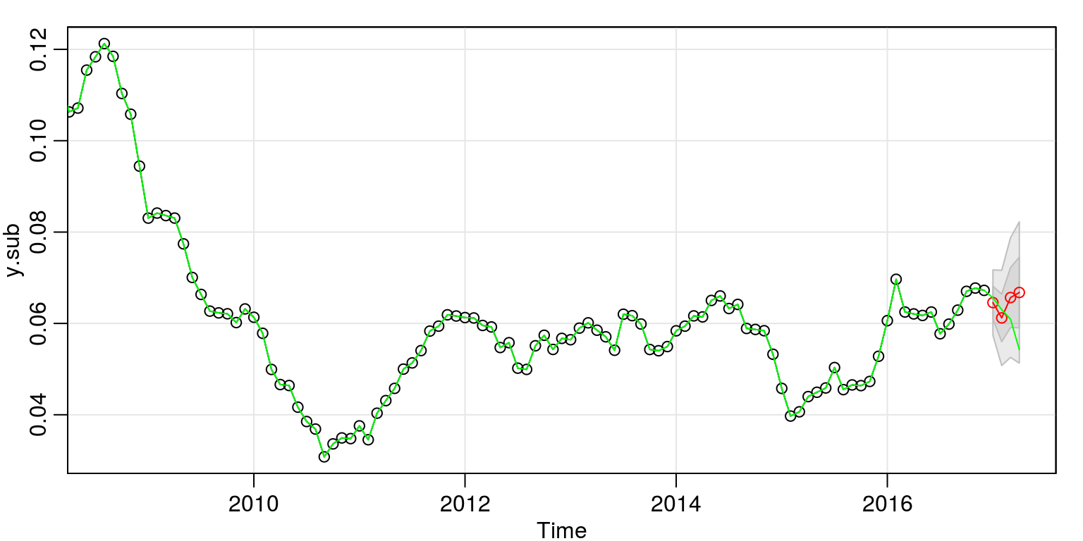
On this occasion the forecast does not look too bad for the one-step ahead horizon.