Tutorial: Forecasting
by Kevin Kotzé
1 The basic setup
To have a look at the first program for this session, please open the file T3_forecast.R that looks to generate a forecast for South African output growth. Once again, the first thing that we do is clear all variables from the current environment and close all the plots. This is performed with the following commands:
rm(list = ls())
graphics.off()
Thereafter, we will load the toolboxes that we need for this session, which include the tsm package from my GitHub account. If you are using your personal machine then these would have been installed during the second tutorial, however, if you are using one of the University machines then you will need to install these packages with the following commands:
devtools::install_github("KevinKotze/tsm")
install.packages("strucchange", repos = "https://cran.rstudio.com/",
    dependencies = TRUE)
install.packages("forecast", repos = "https://cran.rstudio.com/",
    dependencies = TRUE)
The next step is to make sure that you can access the routines in this package by making use of the library command, which would need to be run regardless of the machine that you are using.
library(tsm)
library(strucchange)
library(forecast)
2 Transforming the data
As noted previosuly, South African GDP data has been preloaded in the tsm package, which is numbered KBP6006D. Hence, to retrieve the data from the package and create the object for the series as dat, we execute the following commands:
dat <- sarb_quarter$KBP6006D
dat.tmp <- diff(log(na.omit(dat)) * 100, lag = 1)
head(dat)
## [1] 565040 574255 584836 590609 594892 592293gdp <- ts(dat.tmp, start = c(1960, 2), frequency = 4)Note that the object dat.tmp is the quarter-on-quarter growth rate and the time series object for this variable is labelled gdp. To make sure that these calculations and extractions have been performed correctly, we inspect a plot of the data.
plot.ts(gdp)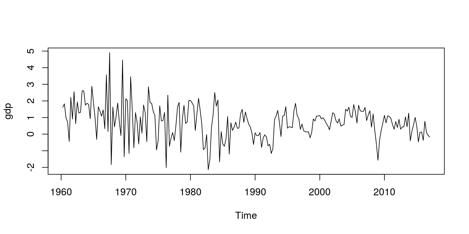
As we did before, we can proceed by checking for structural breaks. In this instance, we once again make use of an AR(1) model and the QLR statistic:
dat.gdp <- cbind(gdp, lag(gdp, k = -1))
colnames(dat.gdp) <- c("ylag0", "ylag1")
dat.gdp <- window(dat.gdp, start = c(1960, 3))
fs <- Fstats(ylag0 ~ ylag1, data = dat.gdp)
breakpoints(fs)
##
## Optimal 2-segment partition:
##
## Call:
## breakpoints.Fstats(obj = fs)
##
## Breakpoints at observation number:
## 42
##
## Corresponding to breakdates:
## 0.1806167sctest(fs, type = "supF")##
## supF test
##
## data: fs
## sup.F = 73.391, p-value = 3.461e-15plot(fs)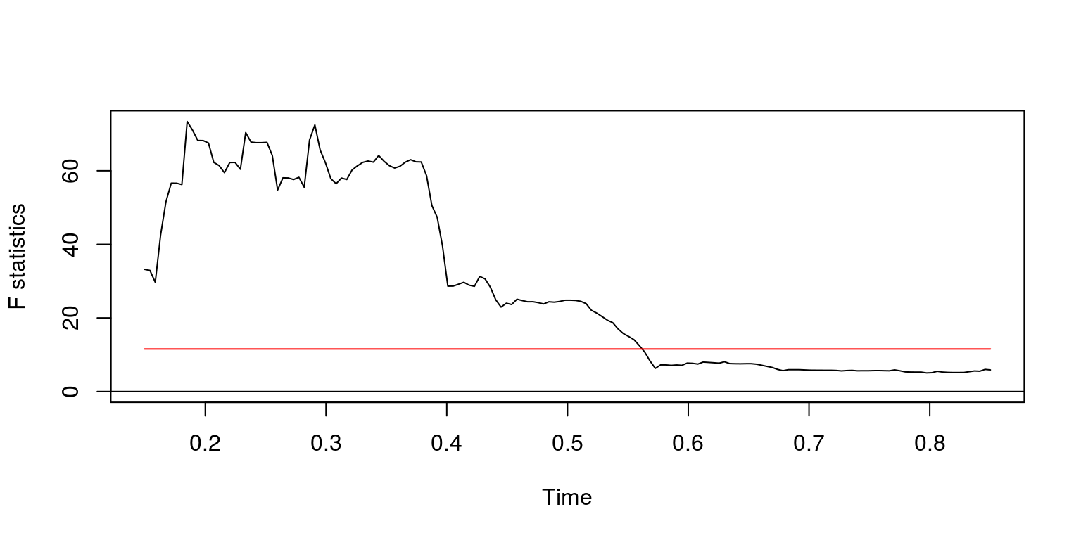
After performing the exercise on successive subsamples of the data, the results suggest that one of the last significant structutral breaks arises towards the end of 1980.
3 Estimating the model parameters
The subsample of the data that starts in 1981 is contained in the y object. To consider the degree of autocorrelation.
y <- window(gdp, start = c(1981, 1))
ac(as.numeric(y))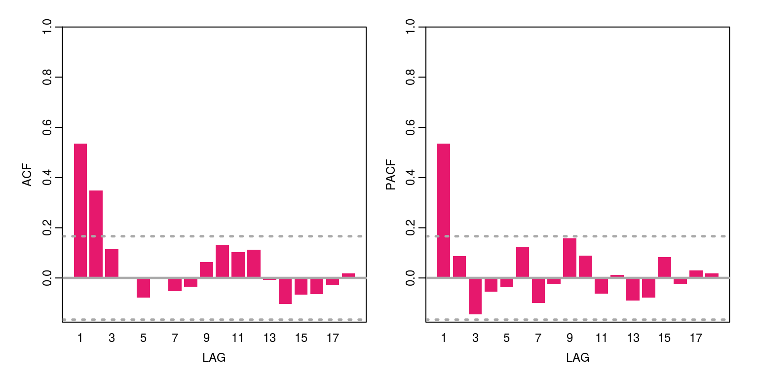
This variable has a bit of persistence and is certainly stationary. The maximum order of this variable is an AR(1) and/or an MA(2). We can then check the information criteria for a number of candidate models by constructing the following vector for the statistics:
arma.res <- rep(0, 8)
arma.res[1] <- arima(y, order = c(1, 0, 2))$aic
arma.res[2] <- arima(y, order = c(1, 0, 1))$aic
arma.res[3] <- arima(y, order = c(1, 0, 0))$aic
arma.res[4] <- arima(y, order = c(0, 0, 2))$aic
arma.res[5] <- arima(y, order = c(0, 0, 1))$aic
To find the model with the smallest AIC value we can then execute the command:
which(arma.res == min(arma.res))## [1] 6 7 8These results suggest that the smallest value is provided by ARMA(1,2). With this in mind we estimate the parameter values for this model structure.
arma <- arima(y, order = c(1, 0, 2))Thereafter, we look at the residuals for the model to determine if there is any serial correlation.
par(mfrow = c(1, 1))
plot(arma$residuals)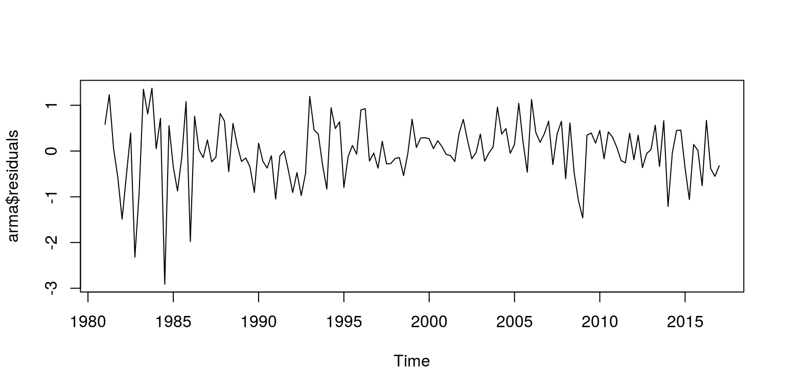
ac(arma$residuals)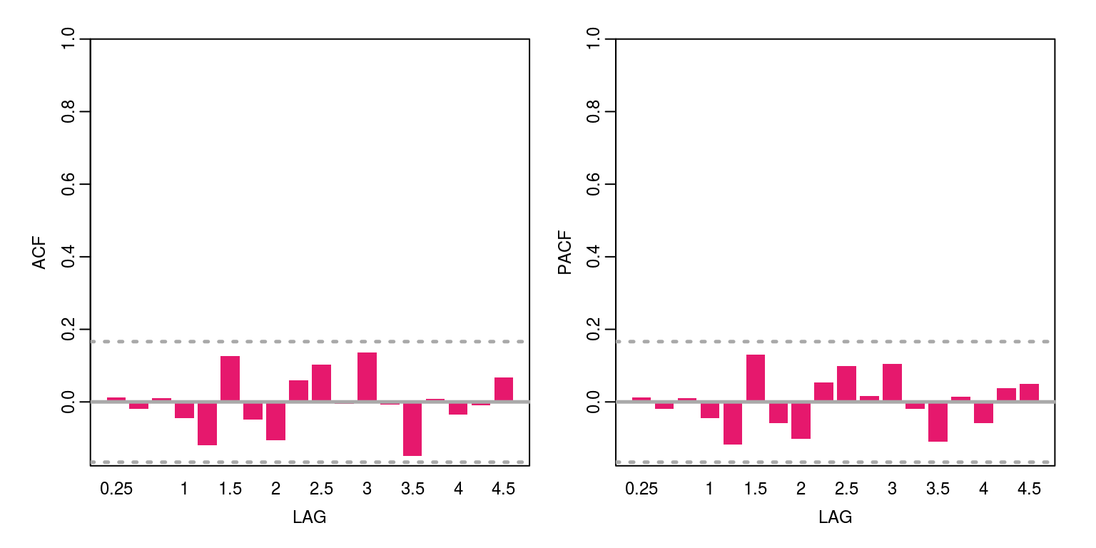
These results suggests that there is no remaining serial correlation.
4 Recursive forecast generation and evaluation
Let us now proceed with a recursive forecasting exercise. What we would like to do is set up a few matrices for the actual data and forecasts, where each row pertains to a subsequent period of time and each column would refer to the additional step ahead forecast. In this exercise, we are going to make use of a forecasting horizon of eight-steps (i.e. two years) and an out-of-sample period of ten-years (i.e. forty observations). Using the notation that was provided in the notes, this would imply that:
H <- 8
P <- 40
obs <- length(y)
R <- obs - (P + H) + 1
To store the actual data that we will use to evaluate the forecast, we need a matrix that has the following dimensions.
actual <- matrix(data = rep(0, P * H), ncol = H)This matrix would need to values that pertain to specific dates. For illustrative purposes, we can substitute the date into each cell with the following commands.
dates <- as.numeric(time(y))
dates[R]  # last initial in-sample observation
## [1] 2005.25for (i in 1:P) {
first <- R + i
last <- first + H - 1
actual[i, 1:H] <- dates[first:last]
}Note that as we move down or to the right, the date increases by one quarter. This is what we want so let’s use actual data now in each of these cells.
actual <- matrix(data = rep(0, P * H), ncol = H)

for (i in 1:P) {
    first <- R + i
    last <- first + H - 1
    actual[i, 1:H] <- y[first:last]
}
We are now going to create a similar matrix to store the forecasts from the ARMA(1,2) model. This matrix would have the following dimensions.
fore.res <- matrix(data = rep(0, P * H), ncol = H)Thereafter, we need to set the subsample for each ARMA(1,2) model. Estimate the parameters with the arima command and forecast eight steps ahead with the predict command. The results will then be stored in the object fore.res.
for (i in 1:P) {
    last.obs <- R + i - 1
    y.sub <- y[1:last.obs]

    arma.est <- arima(y.sub, order = c(1, 0, 2))
    arma.fore <- predict(arma.est, n.ahead = H)

    fore.res[i, 1:H] <- arma.fore$pred
}
To take a look at one of the one- to eight-step ahead forecasts, we can look at what is going on at a particular row of each of these matrices. In this case we have selected the eigth row.
rowf <- 8

par(mfrow = c(1, 1))
plot.ts(actual[rowf, ], col = "black", ylab = "Example",
    xlab = "Steps", ylim = c(min(actual[rowf, ] * 1.5),
        max(actual[rowf, ] * 1.5)))
lines(fore.res[rowf, ], col = "red", lty = 2, lwd = 2)
legend("topright", legend = c("actual", "forecast"), lty = c(1,
    2), col = c("black", "red"), bty = "n")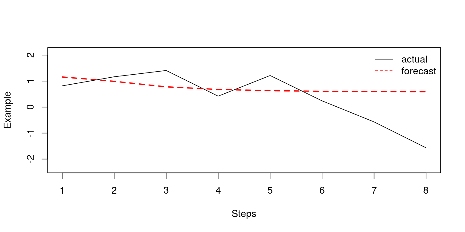
Note that when the horizon is relatively large, the model predictions are particularly poor. It is now relatively easy to create a matrix of similar dimensions that contains the forecast errors.
error <- actual - fore.resTo calculate the average bias at each step ahead, we simply have to find the mean values for each of the columns of the error matrix.
bias.step <- rep(0, H)

for (i in 1:H) {
    bias.step[i] <- mean(error[, i])
}

print(bias.step)
## [1] 0.008407024 0.012181797 0.026870057 -0.013936479
## [5] -0.024702804 -0.054035748 -0.089353974 -0.133394278Note that one average, the model tends to provide a prediction that is too high over the short-run, but too low over the long-run. Similarly, to calculate the bias at each point in time we would simply need to find the mean values for each of the rows in the error matrix.
bias.time <- rep(0, P)

for (i in 1:P) {
    bias.time[i] <- mean(error[i, ])
}

print(bias.time)
## [1] 0.571765956 0.590663472 0.844064294
## [4] 0.487027086 0.447293423 0.354544107
## [7] 0.101853190 -0.363705330 -0.373316729
## [10] -0.524318830 -0.708683129 -0.440880693
## [13] -0.606889392 -0.386817342 0.020491266
## [16] 0.545440208 0.411219668 0.251561128
## [19] 0.225520791 0.070681306 0.173277879
## [22] 0.015862099 -0.086535458 -0.118524536
## [25] 0.012564427 0.081879465 0.052826342
## [28] -0.003203668 -0.153663394 -0.037448319
## [31] 0.038386289 0.021874799 -0.274707016
## [34] -0.221453656 -0.472063350 -0.221369470
## [37] -0.170684325 -0.366835536 -0.578060310
## [40] -0.549458732It is also just as easy to calculate the root-mean squared-error for each step ahead and over time with the aid of the following commands.
RMSE.step <- sqrt(colMeans(error^2))
RMSE.time <- sqrt(rowMeans(error^2))
When we plot the results of the RMSE over time we note that the model forecasts over the global financial crisis were particularly poor. In addition, while the one-step ahead forecast provides a relatively small error, the size of the error increases relatively rapidly until the third-step ahead.
plot(ts(RMSE.time, start = c(2005, 1), frequency = 4), ylab = "RMSE time",
    type = "o", col = "red")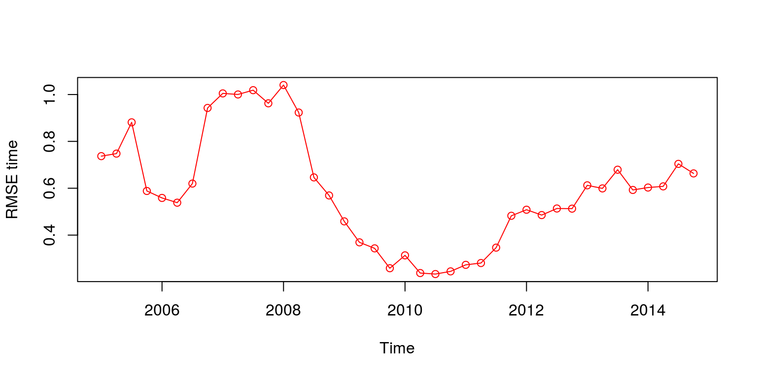
plot(RMSE.step, ylab = "RMSE step", type = "o", col = "red")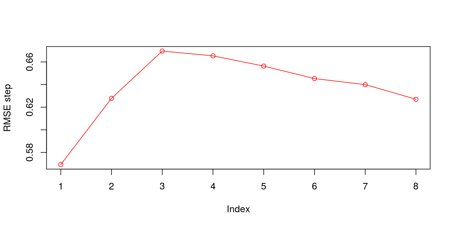
5 Model comparison
In what follows, we are going to consider the results of an alternative forecasting model. The results of the two models could be compared with the aid of the Diebold and Mariano (1995) statistic. Hence, we need to create a matrix for the new set of forecasts that has the same dimensions. In this case we are going to use an AR(1) model to forecast forward.
fore.alt <- matrix(data = rep(0, P * H), ncol = H)

for (i in 1:P) {
    last.obs <- R + i - 1
    y.sub <- y[1:last.obs]

    arma.alt <- arima(y.sub, order = c(1, 0, 0))
    arma.falt <- predict(arma.alt, n.ahead = H)

    fore.alt[i, 1:H] <- arma.falt$pred
}
We can then calculate the forecast errors as well as the RMSE using the routines that have been described above.
error.alt <- fore.alt - actual

RMalt.step <- sqrt(colSums(error.alt^2))  # averaged over time
RMalt.time <- sqrt(rowSums(error.alt^2))  # averaged over all 8 steps
To compare the respective RMSE’s we plot the two results on a common set of axes.
plot.ts(RMSE.step, xlab = "Steps", ylab = "RMSE", ylim = c(min(c(RMSE.step,
    RMalt.step)), max(c(RMSE.step, RMalt.step))))
lines(RMalt.step, col = "red", lty = 2)
legend("topright", legend = c("ARMA(1,2)", "AR(1)"), lty = c(1,
    2), col = c("black", "red"), bty = "n")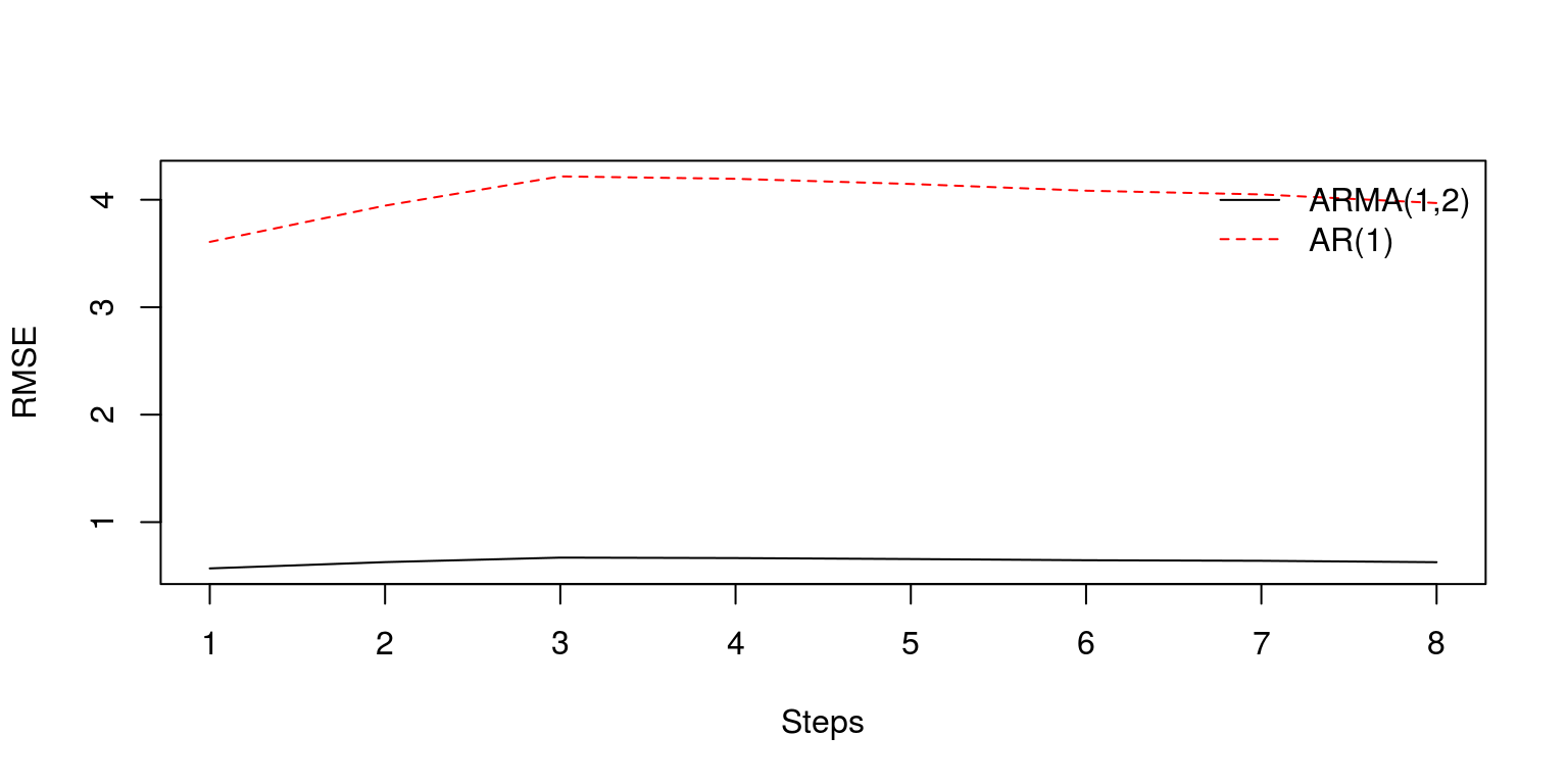
plot(ts(RMSE.time, start = c(2005, 1), frequency = 4), ylab = "RMSE",
    ylim = c(min(c(RMSE.time, RMalt.time)), max(c(RMSE.time,
        RMalt.time))))
lines(ts(RMalt.time, start = c(2005, 1), frequency = 4),
    col = "red", lty = 2)
legend("topright", legend = c("ARMA(1,2)", "AR(1)"), lty = c(1,
    2), col = c("black", "red"), bty = "n")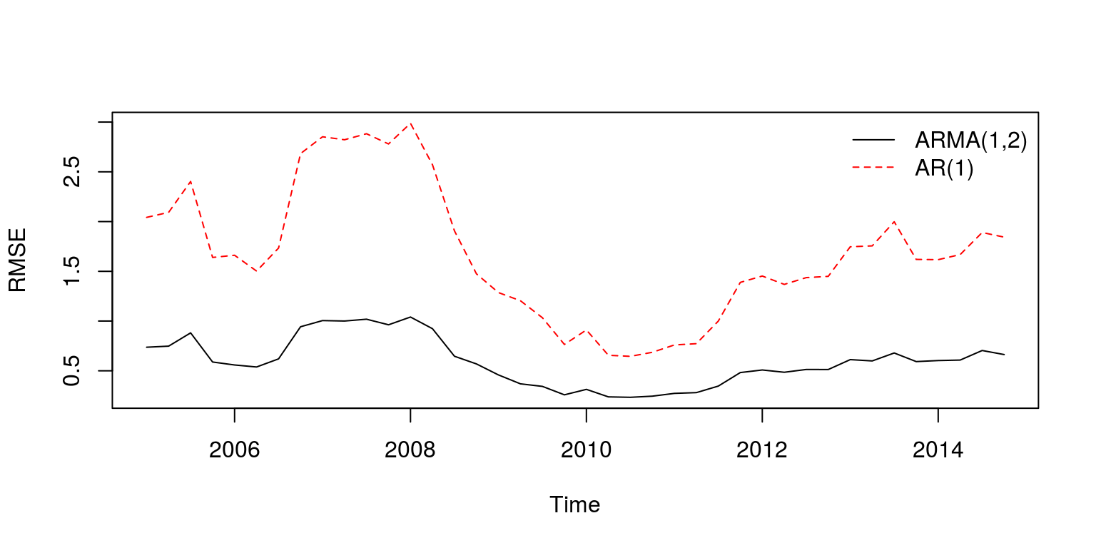
Note that the ARMA(1,2) would clearly appear to provide better forecast estimates. To determine whether the difference between the estimates are significant or not, we can make use of the Diebold and Mariano (1995) statistic. To calculate this statistic for each step ahead, we can create a vector of eight observations and use the dm.test command that is contained in the forecast package.
dm.steps <- rep(0, H)

for (i in 1:H) {
    dm.steps[i] <- dm.test(error[, i], error.alt[, i], h = i)$statistic
}
The easiest way to display these results is with the aid of a simple plot.
plot(dm.steps, ylim = c(-3, 3), xlab = "Steps", ylab = "DM statistic")
lines(rep(0, H), col = "grey", lty = 1)
lines(rep(1.96, H), col = "red", lty = 2)
lines(rep(-1.96, H), col = "red", lty = 2)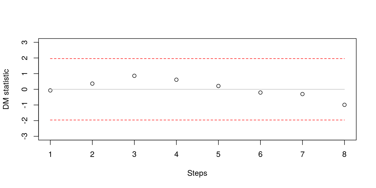
Note that the results are within the confidence bands so the forecasting results are not significantly different from one another. We could also consider the Diebold and Mariano (1995) statistics for each period of time (although this is seldomly performed in most empirical studies). The commands that we use largely follow what has been described above.
dm.time <- rep(0, P)

for (i in 1:P) {
    dm.time[i] <- dm.test(error[i, ], error.alt[i, ], h = 1)$statistic
}

plot(ts(dm.time, start = c(2005, 1), frequency = 4), type = "p",
    ylim = c(-5, 5), ylab = "DM statistic")
lines(ts(rep(0, P), start = c(2005, 1), frequency = 4),
    col = "grey", lty = 1)
lines(ts(rep(1.96, P), start = c(2005, 1), frequency = 4),
    col = "red", lty = 2)
lines(ts(rep(-1.96, P), start = c(2005, 1), frequency = 4),
    col = "red", lty = 2)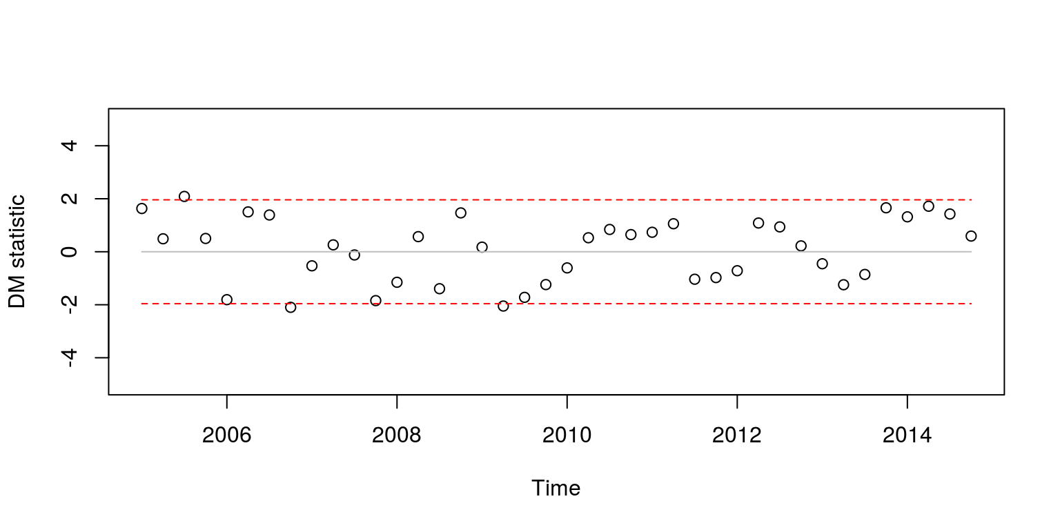
Almost all of the test statistics are within the critical values. As I can never remember, which model pertains to positive values of the statistic I always have a look at the RMSE’s that pertain to particular observations. For example, when we want to see which model produced the lowest RMSE for the third iterative forecast, we simply make use of the following commands.
RMSE.time[3]## [1] 0.8813765RMalt.time[3]## [1] 2.40308This would suggest that the ARMA(1,2) model is significantly better when the DM statistic is above +1.96 and the AR(1) model is significantly better when the DM statistic is below -1.96.
5.1 Comparing nested models
In this case, where the AR(1) is nested within the AR(1,2) we would usually want to use the Clarke-West statistic. This routine is stored within the tsm package. The results for the statistic and corresponding p-value for each step ahead can be stored in vectors, as followings
cwstat.steps <- rep(0, H)
cwpval.steps <- rep(0, H)

for (i in 1:H) {
    cwstat.steps[i] <- cw(error[, i], error.alt[, i], fore.res[,
        i], fore.alt[, i])$test
    cwpval.steps[i] <- cw(error[, i], error.alt[, i], fore.res[,
        i], fore.alt[, i])$pvalue
}
The results of this test can be plotted as before, where:
plot(cwstat.steps, ylim = c(-3, 3), xlab = "Steps", ylab = "CW statistic")
lines(rep(0, H), col = "grey", lty = 1)
lines(rep(1.96, H), col = "red", lty = 2)
lines(rep(-1.96, H), col = "red", lty = 2)
Note that once again, the test statistics are within the confidence intervals. These statistics could also be computed for forecasts that were generated at each point in time.
cwstat.time <- rep(0, P)
cwpval.time <- rep(0, P)

for (i in 1:P) {
    cwstat.time[i] <- cw(error[i, ], error.alt[i, ], fore.res[i,
        ], fore.alt[i, ])$test
    cwpval.time[i] <- cw(error[i, ], error.alt[i, ], fore.res[i,
        ], fore.alt[i, ])$pvalue
}
And these results maybe displayed as follows:
plot(ts(cwstat.time, start = c(2005, 1), frequency = 4),
    type = "p", ylim = c(-5, 5), ylab = "CW statistic")
lines(ts(rep(0, P), start = c(2005, 1), frequency = 4),
    col = "grey", lty = 1)
lines(ts(rep(1.96, P), start = c(2005, 1), frequency = 4),
    col = "red", lty = 2)
lines(ts(rep(-1.96, P), start = c(2005, 1), frequency = 4),
    col = "red", lty = 2)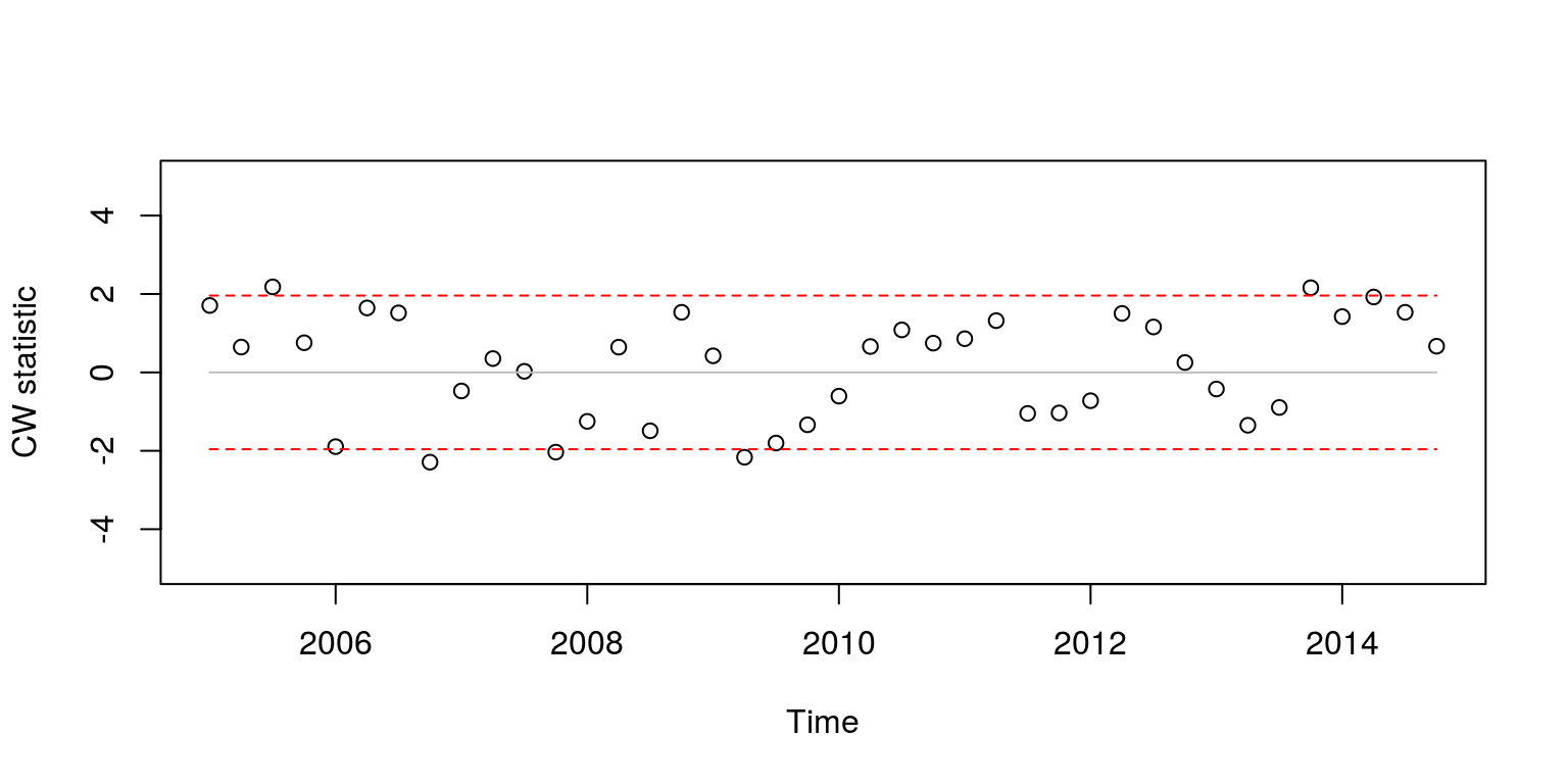
which is similar to what we had before.
6 Constructing a forecast density
The first thing that we would need to do when constructing a forecast density is to set the horizon and intervals. In this case we are going to make use of a sixteen-step ahead forecast and percentiles that take on specific values.
H <- 16
percentiles <- c(0.1, 0.15, 0.25, 0.35)
no.obs <- length(y)
inter <- length(percentiles) * 2
We then need to estimate the model parameters and generate a forecast.
arma.est <- arima(y, order = c(1, 0, 2))
arma.fore <- predict(arma.est, n.ahead = H)
To calculate the density, we make use of information from the forecast mean squared error. These values are all going to be contained in the vector mse.
mse <- rep(0, H)
y.tmp <- y

for (i in 1:H) {
    y.tmp <- c(y.tmp, arma.fore$pred[i])
    mse[i] <- var(y.tmp)
}
Now we need to prepare the fan chart.
fanChart <- matrix(rep(0, H * inter), nrow = H)

for (i in 1:length(percentiles)) {
    z2 <- abs(qnorm(percentiles[i]/2, 0, 1))
    forcInt <- matrix(rep(0, H * 2), ncol = 2)

    for (h in 1:H) {
        forcInt[h, 1] <- arma.fore$pred[h] - z2 * sqrt(mse[h])
        forcInt[h, 2] <- arma.fore$pred[h] + z2 * sqrt(mse[h])

        fanChart[h, i] <- forcInt[h, 1]
        fanChart[h, inter - i + 1] <- forcInt[h, 2]
    }
}
We can then create objects for the respective elements that will find their way onto the plot.
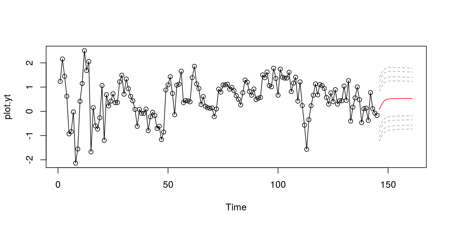
plot.len <- no.obs + H
plot.yt <- c(y, rep(NaN, H))
plot.ytF <- c(rep(NaN, no.obs), arma.fore$pred)
The point forecast estimate can then be plotted, with the corresponding predictive density.
plot.ts(plot.yt, type = "o")
lines(plot.ytF, col = "red", lty = 1)

plot.ytD <- rbind(matrix(rep(NaN, no.obs * inter), ncol = inter),
    fanChart)
no.int <- dim(plot.ytD)

for (i in 1:no.int[2]) {
    lines(plot.ytD[, i], col = "darkgrey", lty = 2)
}
As this does not look very professional, we can make use of the shading with the polygon command in what follows.
start.obs <- no.obs + 1

plot(plot.yt, type = "o", ylim = c(-6, 6), ylab = "", xlab = "")

polygon(c(c(start.obs:plot.len), rev(c(start.obs:plot.len))),
    c(plot.ytD[start.obs:plot.len, 1], rev(plot.ytD[start.obs:plot.len,
        8])), col = "grey90", border = NA)

polygon(c(c(start.obs:plot.len), rev(c(start.obs:plot.len))),
    c(plot.ytD[start.obs:plot.len, 2], rev(plot.ytD[start.obs:plot.len,
        7])), col = "grey80", border = NA)

polygon(c(c(start.obs:plot.len), rev(c(start.obs:plot.len))),
    c(plot.ytD[start.obs:plot.len, 3], rev(plot.ytD[start.obs:plot.len,
        6])), col = "grey70", border = NA)

polygon(c(c(start.obs:plot.len), rev(c(start.obs:plot.len))),
    c(plot.ytD[start.obs:plot.len, 4], rev(plot.ytD[start.obs:plot.len,
        5])), col = "grey60", border = NA)

lines(plot.ytF, col = "red", lty = 1)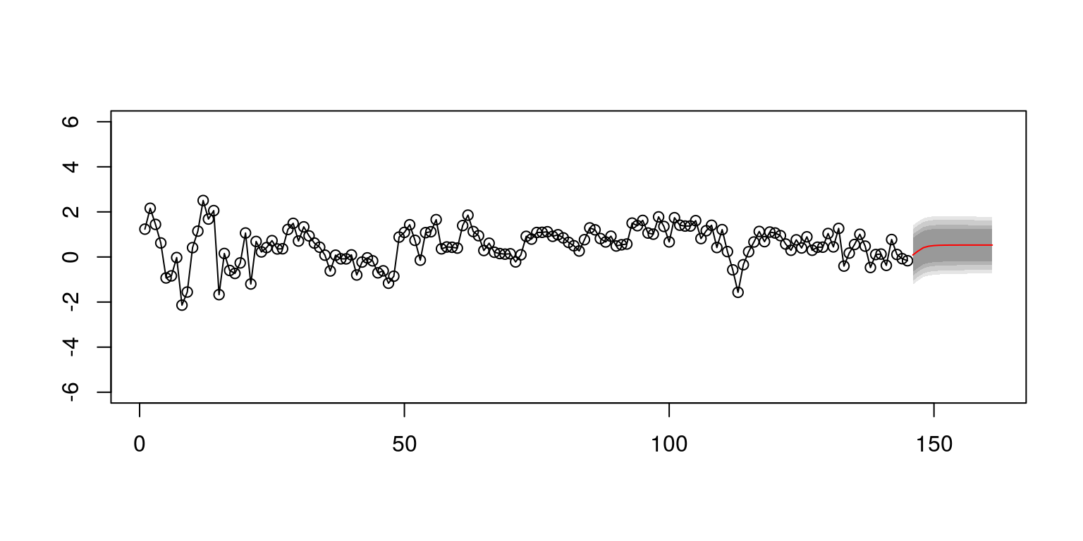
7 Other forecast plots
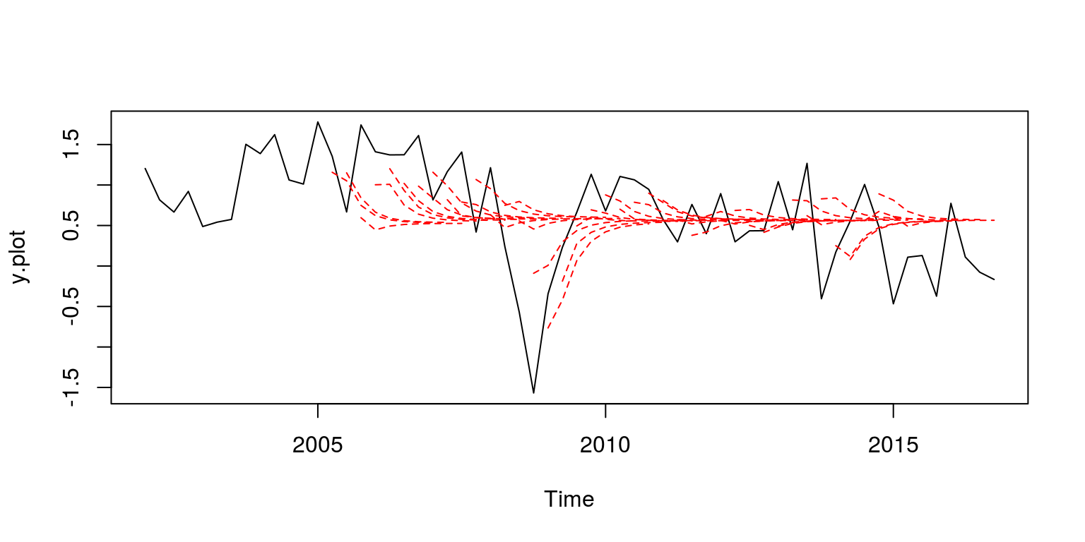
To plot a hairy plot one could make use of the following set of commands.
H <- 8
h.start <- R - 12
dates[h.start]
## [1] 2002.25y.plot <- ts(y[h.start:length(y)], start = c(2002, 1), frequency = 4)
n.obs <- length(y.plot)
no.fore <- n.obs - P - H
nons <- n.obs - H
fore.plot <- matrix(data = rep(0, n.obs * P), nrow = P)
for (i in 1:P) {
nan.beg <- rep(NaN, no.fore + i)
nan.end <- rep(NaN, P - i)
fore.plot[i, 1:n.obs] <- c(nan.beg, fore.res[i, ], nan.end)
}
plot.ts(y.plot)
for (i in 1:P) {
lines(ts(fore.plot[i, ], start = c(2002, 1), frequency = 4),
col = "red", lty = 2)
}