Tutorial: State-Space Modelling
by Kevin Kotzé
1 The local level model
The first program for this session makes use of a local level model that is applied to the measure of the South African GDP deflator. This is contained in the file T4-llm.R. Once again, the first thing that we do is clear all variables from the current environment and close all the plots. This is performed with the following commands:
rm(list = ls())
graphics.off()
Thereafter, we will need to install the dlm package that we will use in this session, as well as the tsm package from my GitHub account. If you are using your personal machine then you would already installed tsm package.
devtools::install_github("KevinKotze/tsm")
install.packages("dlm", repos = "https://cran.rstudio.com/",
    dependencies = TRUE)
The next step is to make sure that you can access the routines in this package by making use of the library command, which would need to be run regardless of the machine that you are using.
library(tsm)
library(dlm)
1.1 Transforming the data
As noted previosuly, South African GDP data has been preloaded in the tsm package. Real GDP is numbered KBP6006D and nominal GDP is KBP6006L. Hence, to retrieve the data from the package and create the object for the GDP deflator that will be stored in dat, we execute the following commands:
dat <- sarb_quarter$KBP6006L/sarb_quarter$KBP6006D
dat.tmp <- diff(log(na.omit(dat)) * 100, lag = 1)
head(dat)
## [1] 0.009372788 0.009321643 0.009274395 0.009434330
## [5] 0.009418516 0.009429455inf <- ts(dat.tmp, start = c(1960, 2), frequency = 4)Note that the object dat.tmp is the quarter-on-quarter measure of inflation, as derived from the GDP deflator. To make sure that these calculations and extractions have been performed correctly, we inspect a plot of the data.
plot.ts(inf)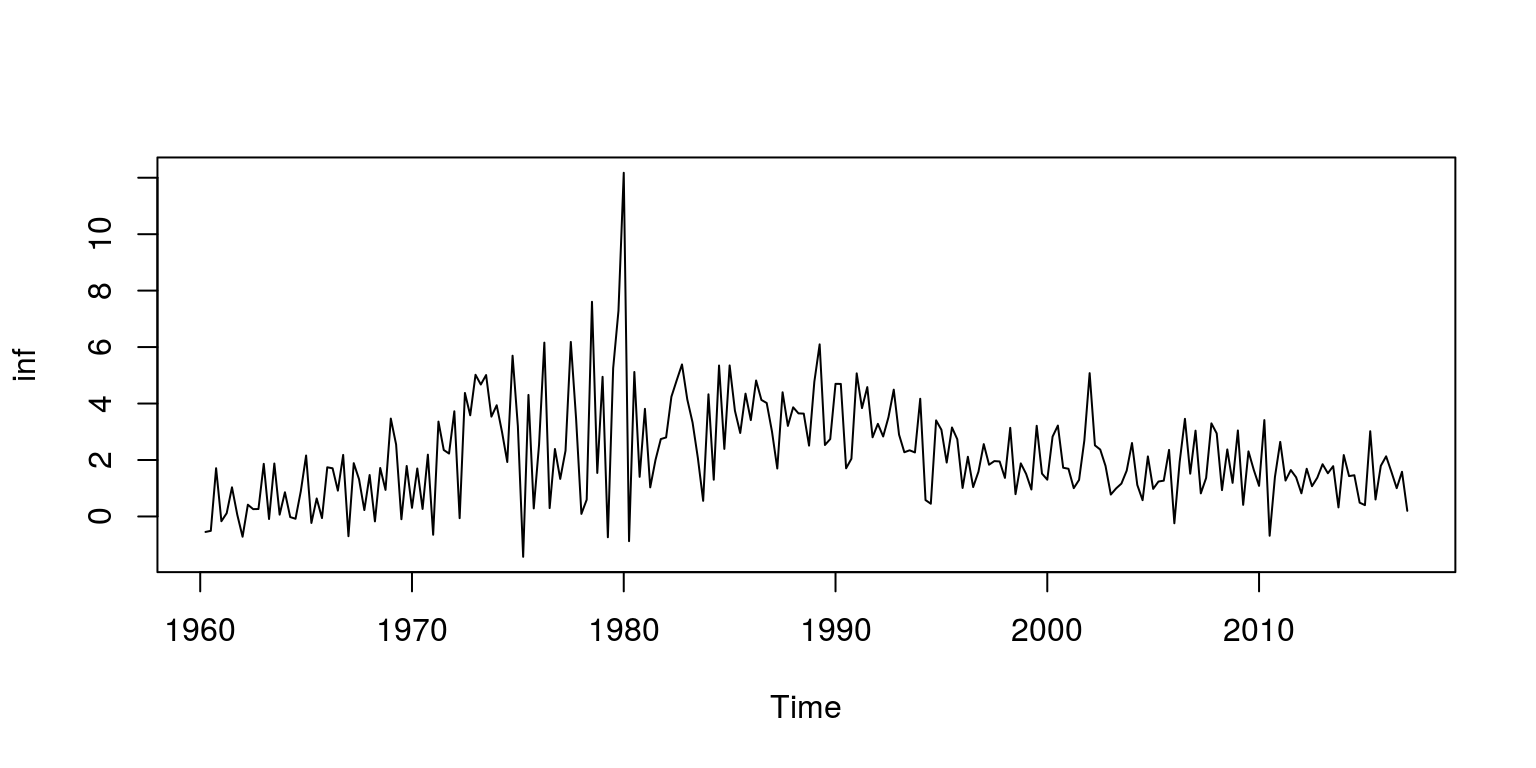
1.2 Construct the model and estimate parameters
As already noted, the first model that we are going to build is a local level model, which includes a stochastic slope. The dlm package has a relatively convenient way to construct these models according to the order of the polynomial, where a first order polynominal is a local level model. We also need to allow for one parameter for the error in the mesurement equation and a second parameter for the error in the solitary state equation. These parameters are labelled parm[1] and parm[2], respectively.
fn <- function(parm) {
    dlmModPoly(order = 1, dV = exp(parm[1]), dW = exp(parm[2]))
}
Thereafter, we are going to assume that the starting values for the parameters are small (i.e. zero) and proceed to fit the model to the data with the aid of maximum-likelihood methods.
fit <- dlmMLE(inf, rep(0, 2), build = fn, hessian = TRUE)
(conv <- fit$convergence)
## [1] 0Note that by placing brackets around the command it will print the result in the console, where we note that convergence has been achieved. We can then construct the likelihood function and generate statistics for the information criteria.
loglik <- dlmLL(inf, dlmModPoly(1))
n.coef <- 2
r.aic <- (2 * (loglik)) + 2 * (sum(n.coef))  #dlmLL caculates the neg. LL
r.bic <- (2 * (loglik)) + (log(length(inf))) * (n.coef)
The statistics for the variance-covariance matrix could also be extracted from the model object with the use of the commands:
mod <- fn(fit$par)
obs.error.var <- V(mod)
state.error.var <- W(mod)
1.3 Kalman filter and smoother
To extract information relating to the Kalman filter and smoother, we use the instructions:
filtered <- dlmFilter(inf, mod = mod)
smoothed <- dlmSmooth(filtered)
Thereafter, we can look at the results from the Kalman filter to derive the measurement errors. These have been stored in the resids object. We could also plot the smoothed values of the stochastic trend, which has been labeled mu.
resids <- residuals(filtered, sd = FALSE)
mu <- dropFirst(smoothed$s)
mu.1 <- mu[1]
mu.end <- mu[length(mu)]
1.4 Plot the results
To plot the results on two graphs, we use the mfrow command to create two rows and one column for the plot area. Thereafter, the first plot includes data for the actual variable and the black line refers to the stochastic trend and the grey line depicts the actual data. The graph below depicts the measurement errors.
par(mfrow = c(2, 1), mar = c(2.2, 2.2, 1, 1), cex = 0.8)
plot.ts(inf, col = "darkgrey", xlab = "", ylab = "", lwd = 1.5)
lines(mu, col = "black")
legend("topright", legend = c("Observed Deflator", "Stochastic level"),
    lwd = c(2, 1), col = c("darkgrey", "black"), bty = "n")

plot.ts(resids, ylab = "", xlab = "", col = "darkgrey",
    lwd = 1.5)
abline(h = 0)
legend("topright", legend = "Residuals", lwd = 1.5, col = "darkgrey",
    bty = "n")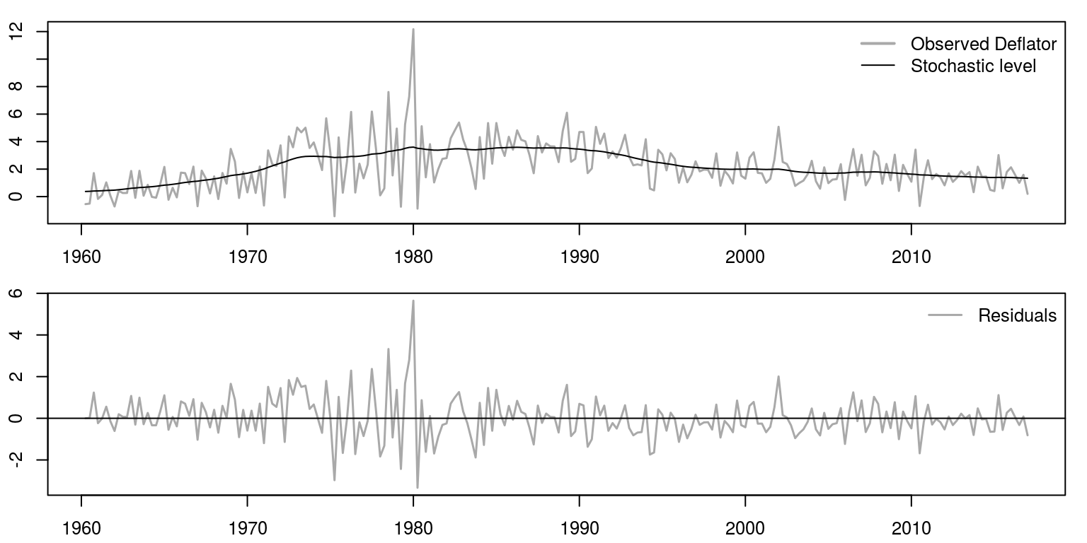
We can also print the results of the information criteria, as well as the variance of the respective errors.
cat("AIC", r.aic)## AIC 530.5972cat("BIC", r.bic)## BIC 537.4559cat("V.variance", obs.error.var)## V.variance 2.166748cat("W.variance", state.error.var)## W.variance 0.02719818The diagnostics of the residuals, which are included below, suggest that there is no evidence of remaining serial correlation and their distribution is relatively normal.
par(mfrow = c(1, 1), mar = c(2.2, 2.2, 1, 1), cex = 0.8)
hist(resids, prob = TRUE, col = "grey", main = "", breaks = seq(-4.5,
    7, length.out = 30))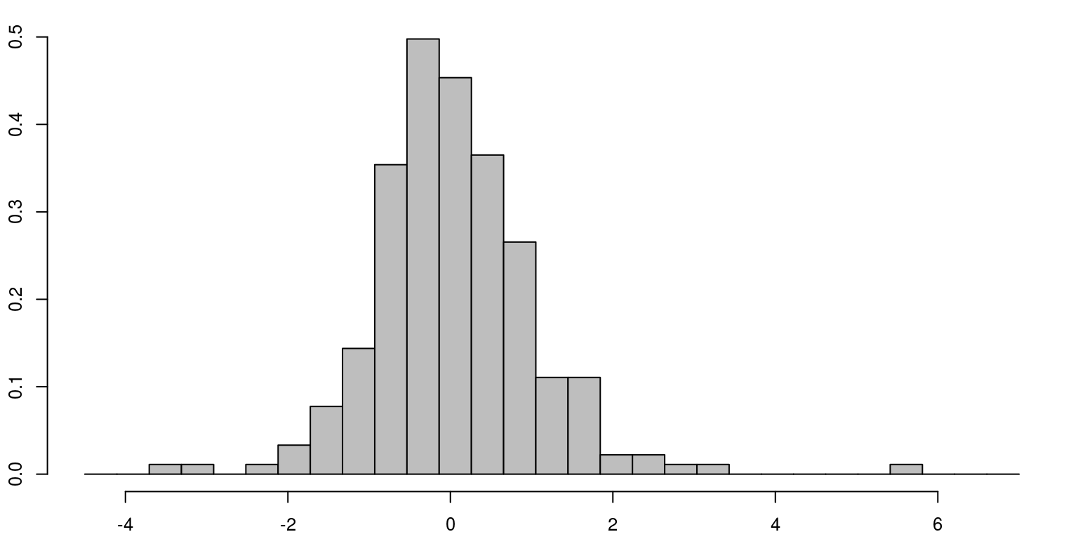
ac(resids) # acf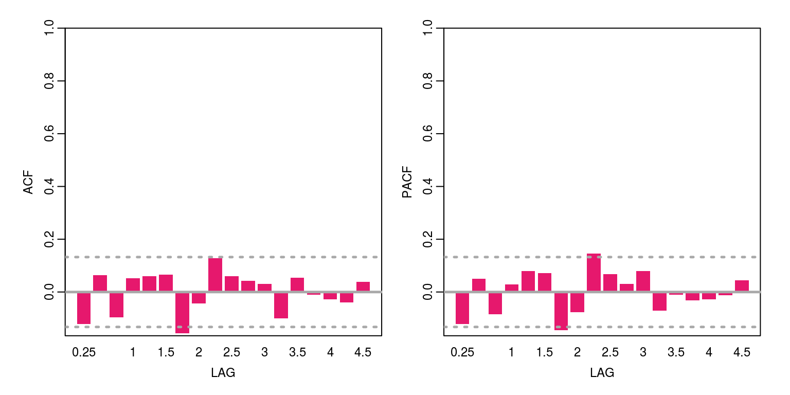
Box.test(resids, lag = 12, type = "Ljung", fitdf = 2) # joint autocorrelation##
## Box-Ljung test
##
## data: resids
## X-squared = 20.598, df = 10, p-value = 0.02408shapiro.test(resids) # normality##
## Shapiro-Wilk normality test
##
## data: resids
## W = 0.94818, p-value = 2.84e-07In this case all appears to be satisfactory, as there is no unexplained autocorrelation when the p-value is less than 5% and the Shapiro test would suggest that the residuals are normally distributed when the p-value is less than 5%.
2 The local level trend model
An example of the local level trend model is contained in the file T4-llm_trend.R. To estimate values for the parameters and unobserved components for this model, we could start off exactly as we did before.
rm(list = ls())
graphics.off()

dat <- sarb_quarter$KBP6006L/sarb_quarter$KBP6006D
dat.tmp <- diff(log(na.omit(dat)) * 100, lag = 1)
head(dat)
inf <- ts(dat.tmp, start = c(1960, 2), frequency = 4)
plot.ts(inf)
2.1 Construct the model and estimate parameters
However, in this case we need to incorporate an additional state equation for the slope of the model. This is a second order polynomial model and as there are two independent stochastic errors we also need to include this feature in the model.
fn <- function(parm) {
    dlmModPoly(order = 2, dV = exp(parm[1]), dW = exp(parm[2:3]))
}
We can then calculate the information criteria in the same way that we did previously, using the following commands.
fit <- dlmMLE(inf, rep(0, 3), build = fn, hessian = TRUE)
conv <- fit$convergence  # zero for converged

loglik <- dlmLL(inf, dlmModPoly(2))
n.coef <- 3
r.aic <- (2 * (loglik)) + 2 * (sum(n.coef))  #dlmLL caculates the neg. LL
r.bic <- (2 * (loglik)) + (log(length(inf))) * (n.coef)

mod <- fn(fit$par)
obs.error.var <- V(mod)
state.error.var <- diag(W(mod))
2.2 Kalman filter and smoother
The values for the Kalman filter and smoother could also be extracted as before, but note that in this case we are also interested in the values of the stochastic slope, which is allocated to the upsilon object.
filtered <- dlmFilter(inf, mod = mod)
smoothed <- dlmSmooth(filtered)
resids <- residuals(filtered, sd = FALSE)
mu <- dropFirst(smoothed$s[, 1])
upsilon <- dropFirst(smoothed$s[, 2])
mu.1 <- mu[1]
mu.end <- mu[length(mu)]
ups.1 <- upsilon[1]
ups.end <- upsilon[length(mu)]
2.3 Plot the results
We are now going to plot the results for the three graphs underneath one another, using the commands.
par(mfrow = c(3, 1), mar = c(2.2, 2.2, 1, 1), cex = 0.8)
plot.ts(inf, col = "darkgrey", xlab = "", ylab = "", lwd = 2)
lines(mu, col = "black")
legend("topright", legend = c("Observed Deflator", "Stochastic level"),
    lwd = c(2, 1), col = c("darkgrey", "black"), bty = "n")

plot.ts(upsilon, col = "darkgrey", xlab = "", ylab = "",
    lwd = 2)
legend("topright", legend = "Slope", lwd = 2, col = "darkgrey",
    bty = "n")

plot.ts(resids, ylab = "", xlab = "", col = "darkgrey",
    lwd = 2)
abline(h = 0)
legend("topright", legend = "Residuals", lwd = 2, col = "darkgrey",
    bty = "n")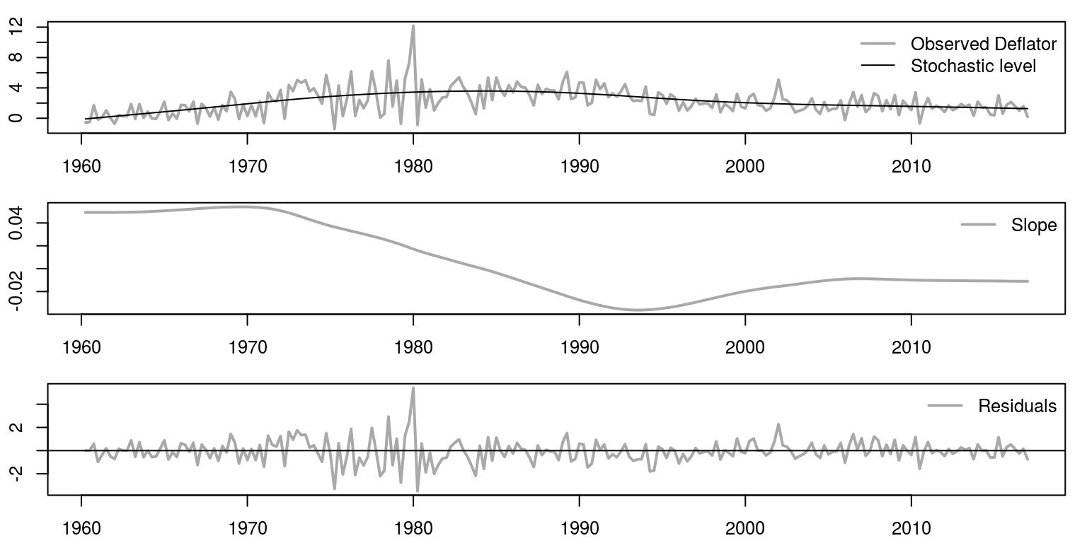
We can also print the results of the information criteria, as well as the variance of the respective errors.
cat("AIC", r.aic)## AIC 696.84cat("BIC", r.bic)## BIC 707.1281cat("V.variance", obs.error.var)## V.variance 2.20686cat("W.variance", state.error.var)## W.variance 1.271627e-08 2.915101e-05The diagnostics of the residuals, which are included below, suggest that there is no evidence of remaining serial correlation and their distribution is relatively normal.
ac(resids) # acf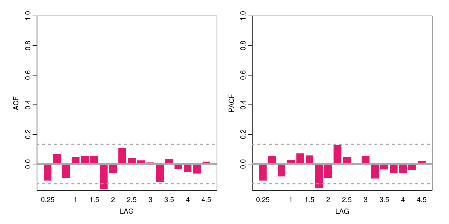
Box.test(resids, lag = 12, type = "Ljung", fitdf = 2) # joint autocorrelation##
## Box-Ljung test
##
## data: resids
## X-squared = 18.924, df = 10, p-value = 0.04123shapiro.test(resids) # normality##
## Shapiro-Wilk normality test
##
## data: resids
## W = 0.95141, p-value = 6.09e-073 The local level model with seasonal
An example of the local level trend model is contained in the file T4-llm_seas.R. To estimate values for the parameters and unobserved components in this model we could start off exactly as we did before.
rm(list = ls())
graphics.off()

dat <- sarb_quarter$KBP6006L/sarb_quarter$KBP6006D
dat.tmp <- diff(log(na.omit(dat)) * 100, lag = 1)
head(dat)
inf <- ts(dat.tmp, start = c(1960, 2), frequency = 4)
plot.ts(inf)
3.1 Construct the model and estimate parameters
However, in this case we need to incorporate an additional state equations for the seasonal components. This is a first order polynomial model with the additional seasonal component that is measured at a quarterly frequency.
fn <- function(parm) {
    mod <- dlmModPoly(order = 1) + dlmModSeas(frequency = 4)
    V(mod) <- exp(parm[1])
    diag(W(mod))[1:2] <- exp(parm[2:3])
    return(mod)
}
We can then calculate the information criteria in the same way that we did previously, using the following commands.
fit <- dlmMLE(inf, rep(0, 3), build = fn, hessian = TRUE)
conv <- fit$convergence  # zero for converged

loglik <- dlmLL(inf, dlmModPoly(1) + dlmModSeas(4))
n.coef <- 3
r.aic <- (2 * (loglik)) + 2 * (sum(n.coef))  #dlmLL caculates the neg. LL
r.bic <- (2 * (loglik)) + (log(length(inf))) * (n.coef)

mod <- fn(fit$par)
obs.error.var <- V(mod)
state.error.var <- diag(W(mod))
3.2 Kalman filter and smoother
The values for the Kalman filter and smoother could also be extracted as before, but note that in this case we are also interested in the values of the seasonal, which is allocated to the gamma object.
filtered <- dlmFilter(inf, mod = mod)
smoothed <- dlmSmooth(filtered)
resids <- residuals(filtered, sd = FALSE)
mu <- dropFirst(smoothed$s[, 1])
gammas <- dropFirst(smoothed$s[, 2])
mu.1 <- mu[1]
mu.end <- mu[length(mu)]
gammas.1 <- gammas[1]
gammas.end <- gammas[length(mu)]
3.3 Plot the results
We are now going to plot the results for the three graphs underneath one another, using the commands.
par(mfrow = c(3, 1), mar = c(2.2, 2.2, 1, 1), cex = 0.8)
plot.ts(inf, col = "darkgrey", xlab = "", ylab = "", lwd = 2)
lines(mu, col = "black")
legend("topright", legend = c("Observed Deflator", "Stochastic level"),
    lwd = c(2, 1), col = c("darkgrey", "black"), bty = "n")

plot.ts(gammas, col = "darkgrey", xlab = "", ylab = "",
    lwd = 2)
legend("topright", legend = "Seasonal", lwd = 2, col = "darkgrey",
    bty = "n")

plot.ts(resids, ylab = "", xlab = "", col = "darkgrey",
    lwd = 2)
abline(h = 0)
legend("topright", legend = "Residuals", lwd = 2, col = "darkgrey",
    bty = "n")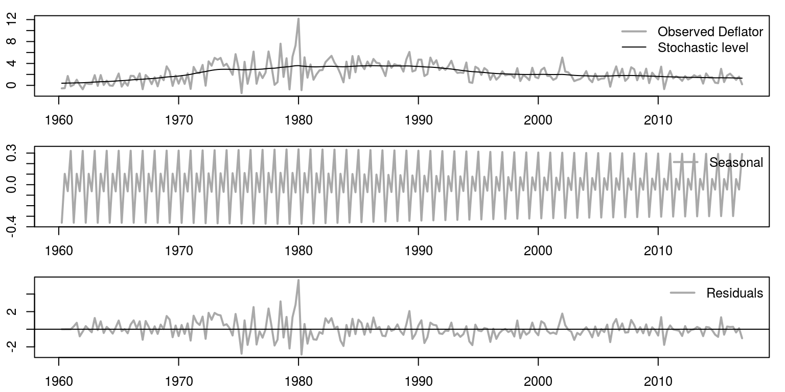
Of course, as these model elements are additive, we could combine the seasonal and the level, as in the following graph.
par(mfrow = c(1, 1), mar = c(2.2, 2.2, 1, 1), cex = 0.8)
alpha <- mu + gammas
par(mfrow = c(1, 1), mar = c(2.2, 2.2, 1, 1), cex = 0.8)
plot.ts(inf, col = "darkgrey", xlab = "", ylab = "", lwd = 2)
lines(alpha, col = "black")
legend("topright", legend = c("Observed Deflator", "State Components"),
    lwd = c(2, 1), col = c("darkgrey", "black"), bty = "n")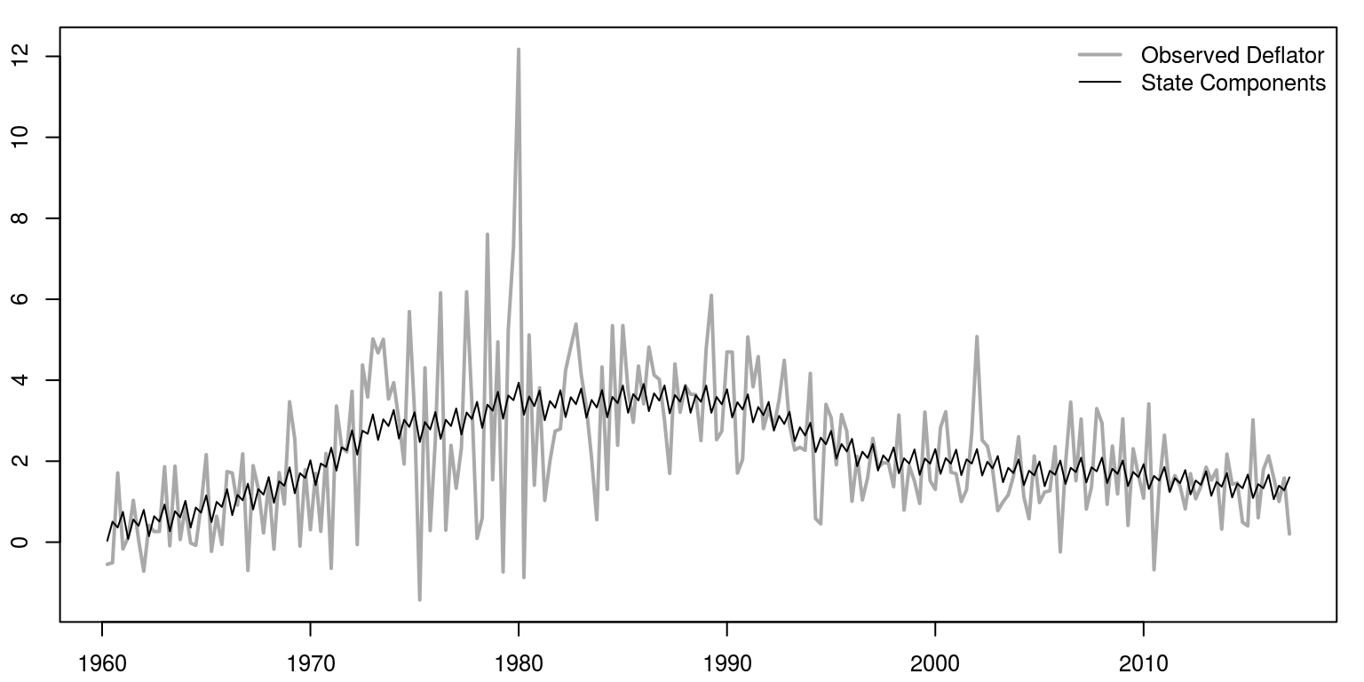
We can also print the results of the information criteria, as well as the variance of the respective errors.
cat("AIC", r.aic)## AIC 646.7115cat("BIC", r.bic)## BIC 656.9995cat("V.variance", obs.error.var)## V.variance 2.13123cat("W.variance", state.error.var)## W.variance 0.02726813 0.0002536817 0 0The diagnostics of the residuals, which are included below, suggest that there is no evidence of remaining serial correlation and their distribution is relatively normal.
ac(resids) # acf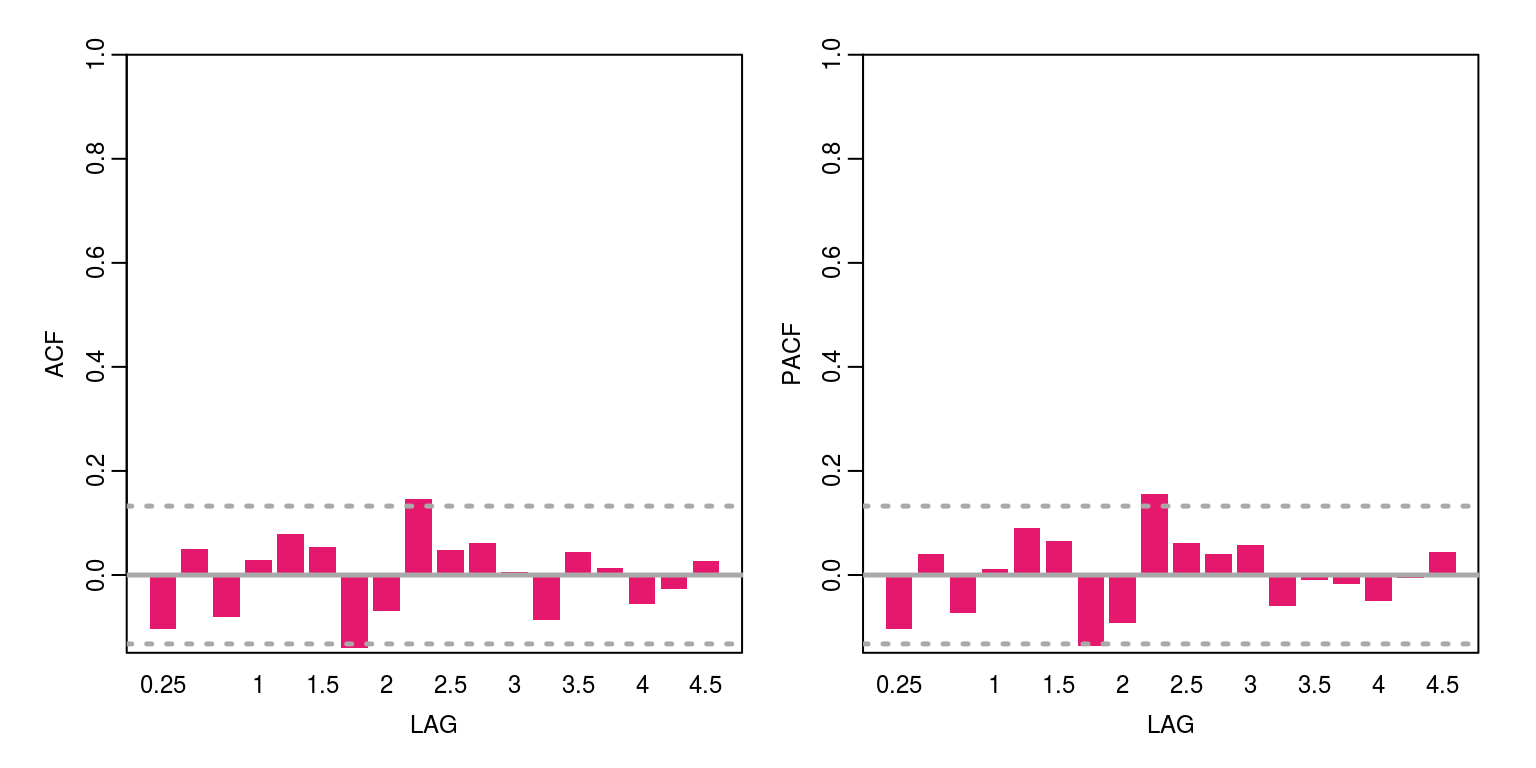
Box.test(resids, lag = 12, type = "Ljung", fitdf = 2) # joint autocorrelation##
## Box-Ljung test
##
## data: resids
## X-squared = 19.304, df = 10, p-value = 0.03657shapiro.test(resids) # normality##
## Shapiro-Wilk normality test
##
## data: resids
## W = 0.95293, p-value = 8.809e-074 Confidence intervals
To create confidence intervals around the estimates from the Kalman filter or smoother, we can use the example of the local level model. An example of a local level model with confidence intervals is contained in T4-llm_conf.R, which contains the following commands:
rm(list = ls())
graphics.off()

dat <- sarb_quarter$KBP6006L/sarb_quarter$KBP6006D
dat.tmp <- diff(log(na.omit(dat)) * 100, lag = 1)
head(dat)
inf <- ts(dat.tmp, start = c(1960, 2), frequency = 4)
plot.ts(inf)
Thereafter, we can use the same model structure that we had originally.
fn <- function(parm) {
    dlmModPoly(order = 1, dV = exp(parm[1]), dW = exp(parm[2]))
}

fit <- dlmMLE(inf, rep(0, 2), build = fn, hessian = TRUE)
conv <- fit$convergence  # zero for converged

loglik <- dlmLL(inf, dlmModPoly(1))
n.coef <- 2
r.aic <- (2 * (loglik)) + 2 * (sum(n.coef))  #dlmLL caculates the neg. LL
r.bic <- (2 * (loglik)) + (log(length(inf))) * (n.coef)

mod <- fn(fit$par)
obs.error.var <- V(mod)
state.error.var <- W(mod)

filtered <- dlmFilter(inf, mod = mod)
smoothed <- dlmSmooth(filtered)
resids <- residuals(filtered, sd = FALSE)
mu <- dropFirst(smoothed$s)
mu.1 <- mu[1]
mu.end <- mu[length(mu)]
4.1 Constructing confidence intervals
To constrct the confidence intervals around the smoothed stochastic trend, we would invoke the commands:
conf.tmp <- unlist(dlmSvd2var(smoothed$U.S, smoothed$D.S))
conf <- ts(as.numeric(conf.tmp)[-1], start = c(1960, 2),
    frequency = 4)
wid <- qnorm(0.05, lower = FALSE) * sqrt(conf)

conf.pos <- mu + wid
conf.neg <- mu - wid
Similarly, if we wanted to do the same for the filtered values we would utilise information relating to the prediction errors.
mu.f <- dropFirst(filtered$a)
cov.tmp <- unlist(dlmSvd2var(filtered$U.R, filtered$D.R))
if (sum(dim(mod$FF)) == 2) {
    variance <- cov.tmp + as.numeric(V(mod))
} else {
    variance <- (sapply(cov.tmp, function(x) mod$FF %*%
        x %*% t(mod$FF))) + V(mod)
}
4.2 Plotting the results
This would allow us to plot the results
par(mfrow = c(1, 1), mar = c(2.2, 2.2, 1, 1), cex = 0.8)
plot.ts(inf, col = "darkgrey", xlab = "", ylab = "", lwd = 1.5)
lines(mu, col = "black")
lines(conf.pos, col = "red")
lines(conf.neg, col = "red")
legend("topright", legend = c("Observed Deflator", "Stochastic level",
    "Confidence Interval"), lwd = c(1.5, 1, 1), col = c("darkgrey",
    "black", "red"), bty = "n")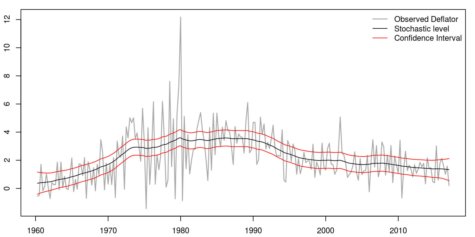
5 Intervention variables
To incorporate a dummy variable we will use the example of the local level model once again. Such an example is contained in the file T4-llm_int.R.
rm(list = ls())
graphics.off()

dat <- sarb_quarter$KBP6006L/sarb_quarter$KBP6006D
dat.tmp <- diff(log(na.omit(dat)) * 100, lag = 1)
head(dat)
inf <- ts(dat.tmp, start = c(1960, 2), frequency = 4)
plot.ts(inf)
To then create the dummy variable we create a vector of zeros that is called lambda, which is the same length as the sample of data. We then include a value of 1 for the first two quarters in 1980 (which relates to observation 79 and 80). This vector of values is then transformed to a time series object.
lambda <- rep(0, length(inf))
lambda[79:80] <- 1
lambda <- ts(lambda, start = c(1960, 2), frequency = 4)
plot(lambda)
The model structure needs to incorporate this dummy variable, which is an additional regressor in the measurement equation. The rest of the code is pretty straightforward and is largely as it was before.
fn <- function(parm) {
    mod <- dlmModPoly(order = 1) + dlmModReg(lambda, addInt = FALSE)
    V(mod) <- exp(parm[1])
    diag(W(mod))[1] <- exp(parm[2])
    return(mod)
}

fit <- dlmMLE(inf, rep(0, 2), build = fn, hessian = TRUE)
conv <- fit$convergence  # zero for converged

loglik <- dlmLL(inf, dlmModPoly(1) + dlmModReg(lambda, addInt = FALSE))
n.coef <- 2
r.aic <- (2 * (loglik)) + 2 * (sum(n.coef))  #dlmLL caculates the neg. LL
r.bic <- (2 * (loglik)) + (log(length(inf))) * (n.coef)

mod <- fn(fit$par)
obs.error.var <- V(mod)
state.error.var <- W(mod)

filtered <- dlmFilter(inf, mod = mod)
smoothed <- dlmSmooth(filtered)
resids <- residuals(filtered, sd = FALSE)
mu <- dropFirst(smoothed$s[, 1])
mu.1 <- mu[1]
mu.end <- mu[length(mu)]
5.1 Plotting the results
The plotting of the results would also be very similar to what we had previously.
par(mfrow = c(2, 1), mar = c(2.2, 2.2, 1, 1), cex = 0.8)
plot.ts(inf, col = "darkgrey", xlab = "", ylab = "", lwd = 2)
lines(mu, col = "black")
legend("topright", legend = c("Observed Deflator", "Stochastic level"),
    lwd = c(2, 1), col = c("darkgrey", "black"), bty = "n")

plot.ts(resids, ylab = "", xlab = "", col = "darkgrey",
    lwd = 2)
abline(h = 0)
legend("topright", legend = "Residuals", lwd = 2, col = "darkgrey",
    bty = "n")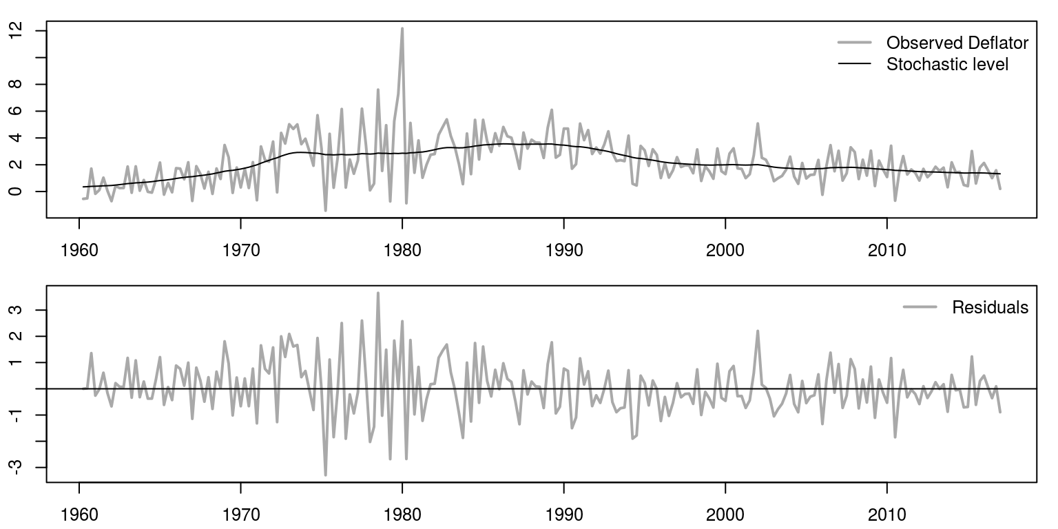
6 Forecasting
To use the model to forecast forward, consider the example that is contained in the file T4-llm_fore.R. The initial lines of code are exactly the same as what we’ve had all along.
rm(list = ls())
graphics.off()

dat <- sarb_quarter$KBP6006L/sarb_quarter$KBP6006D
dat.tmp <- diff(log(na.omit(dat)) * 100, lag = 1)
head(dat)
inf <- ts(dat.tmp, start = c(1960, 2), frequency = 4)
plot.ts(inf)
We can use a local level model structure again, which may be constructed as before, where we include confidence intervals.
fn <- function(parm) {
    dlmModPoly(order = 1, dV = exp(parm[1]), dW = exp(parm[2]))
}

fit <- dlmMLE(inf, rep(0, 2), build = fn, hessian = TRUE)
conv <- fit$convergence  # zero for converged

loglik <- dlmLL(inf, dlmModPoly(1))
n.coef <- 2
r.aic <- (2 * (loglik)) + 2 * (sum(n.coef))  #dlmLL caculates the neg. LL
r.bic <- (2 * (loglik)) + (log(length(inf))) * (n.coef)

mod <- fn(fit$par)
obs.error.var <- V(mod)
state.error.var <- W(mod)

filtered <- dlmFilter(inf, mod = mod)
smoothed <- dlmSmooth(filtered)
resids <- residuals(filtered, sd = FALSE)
mu <- dropFirst(smoothed$s)

conf.tmp <- unlist(dlmSvd2var(smoothed$U.S, smoothed$D.S))
conf <- ts(conf.tmp[-1], start = c(1960, 2), frequency = 4)
wid <- qnorm(0.05, lower = FALSE) * sqrt(conf)

conf.pos <- mu + wid
conf.neg <- mu - wid

comb.state <- cbind(mu, conf.pos, conf.neg)
To forecast forward we use the dlmForecast command, where in this case we are interested in forecasting ten steps ahead.
forecast <- dlmForecast(filtered, nAhead = 12)
var.2 <- unlist(forecast$Q)
wid.2 <- qnorm(0.05, lower = FALSE) * sqrt(var.2)
comb.fore <- cbind(forecast$f, forecast$f + wid.2, forecast$f -
    wid.2)

result <- ts(rbind(comb.state, comb.fore), start = c(1960,
    2), frequency = 4)
6.1 Plotting the results
To draw a graph that contains the results, we would utilise the following commands:
par(mfrow = c(1, 1), mar = c(2.2, 2.2, 1, 1), cex = 0.8)
plot.ts(result, col = c("black", "red", "red"), plot.type = "single",
    xlab = "", ylab = "", lty = c(1, 2, 2), ylim = c(-2,
        8))
lines(inf, col = "darkgrey", lwd = 1.5)
abline(v = c(2014, 1), col = "blue", lwd = 1, lty = 3)
legend("topleft", legend = c("Observed Deflator", "Stochastic level"),
    lwd = c(1.5, 1), col = c("darkgrey", "black"), bty = "n")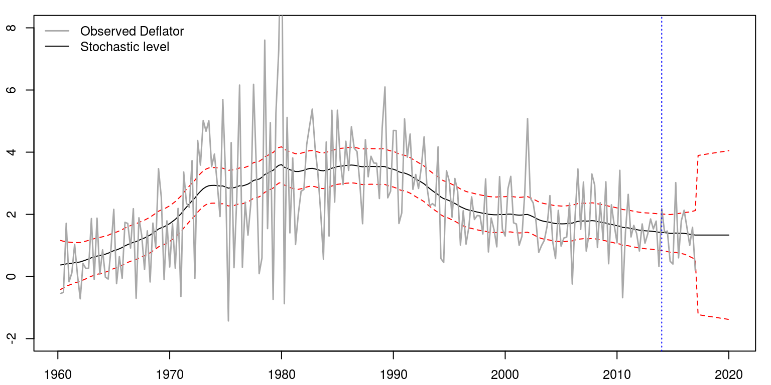
7 Missing data
To model data that has a number of missing observations, consider the example that is contained in the file T4-llm_miss.R. The initial lines of code are exactly the same as what we’ve had all along.
rm(list = ls())
graphics.off()

dat <- sarb_quarter$KBP6006L/sarb_quarter$KBP6006D
dat.tmp <- diff(log(na.omit(dat)) * 100, lag = 1)
head(dat)
inf <- ts(dat.tmp, start = c(1960, 2), frequency = 4)
plot.ts(inf)
To remove some data from the time series for inflation, we can set a number of observations equal to NA, which in this case relates to observations 70 to 82.
inf.mis <- inf
inf.mis[70:82] <- NA
plot(inf.mis)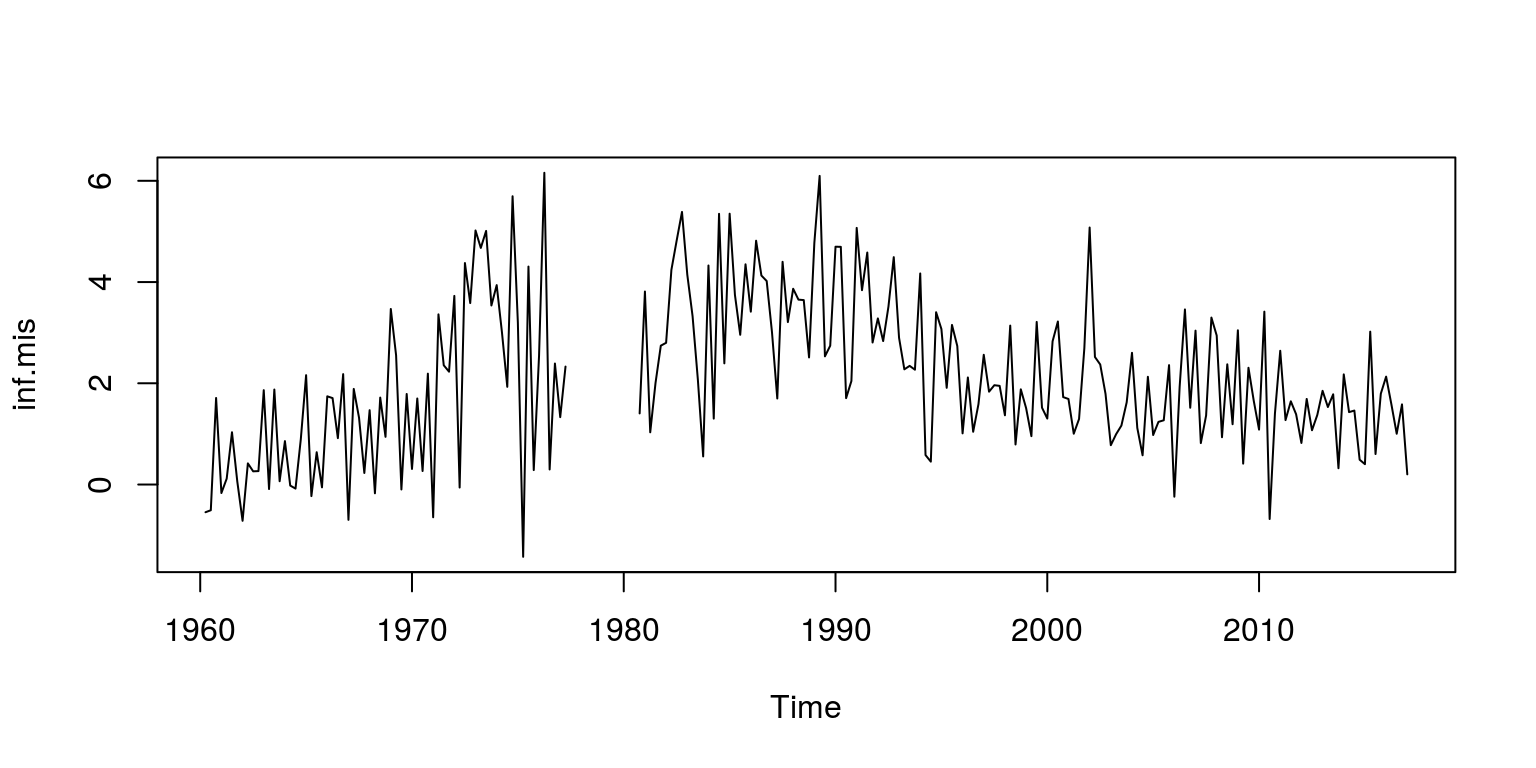
We can use a local level model structure again, which may be constructed as before, where the model will now be applied to the variable inf.mis.
fn <- function(parm) {
    dlmModPoly(order = 1, dV = exp(parm[1]), dW = exp(parm[2]))
}

## Estimate parameters & generate statistics
fit <- dlmMLE(inf.mis, rep(0, 2), build = fn, hessian = TRUE)
conv <- fit$convergence  # zero for converged

loglik <- dlmLL(inf.mis, dlmModPoly(1))
n.coef <- 2
r.aic <- (2 * (loglik)) + 2 * (sum(n.coef))  #dlmLL caculates the neg. LL
r.bic <- (2 * (loglik)) + (log(length(inf))) * (n.coef)

mod <- fn(fit$par)
obs.error.var <- V(mod)
state.error.var <- W(mod)

filtered <- dlmFilter(inf.mis, mod = mod)
smoothed <- dlmSmooth(filtered)
resids <- residuals(filtered, sd = FALSE)
mu <- dropFirst(smoothed$s)

conf.tmp <- dlmSvd2var(smoothed$U.S, smoothed$D.S)
conf <- ts(as.numeric(conf.tmp)[-1], start = c(1960, 2),
    frequency = 4)
wid <- qnorm(0.05, lower = FALSE) * sqrt(conf)

conf.pos <- mu + wid
conf.neg <- mu - wid

comb.state <- cbind(mu, conf.pos, conf.neg)

cat("AIC", r.aic)
## AIC 401.036cat("BIC", r.bic)## BIC 407.8947cat("V.variance", obs.error.var)## V.variance 1.365551cat("W.variance", state.error.var)## W.variance 0.03032414To forecast forward we use the dlmForecast command, where in this case we are interested in forecasting ten steps ahead.
forecast <- dlmForecast(filtered, nAhead = 12)
var.2 <- unlist(forecast$Q)
wid.2 <- qnorm(0.05, lower = FALSE) * sqrt(var.2)
comb.fore <- cbind(forecast$f, forecast$f + wid.2, forecast$f -
    wid.2)

result <- ts(rbind(comb.state, comb.fore), start = c(1960,
    2), frequency = 4)
7.1 Plotting the results
To draw a graph that contains the results, we would utilise the following commands:
par(mfrow = c(1, 1), mar = c(2.2, 2.2, 1, 1), cex = 0.8)
plot.ts(comb.state, col = c("black", "red", "red"), plot.type = "single",
    xlab = "", ylab = "", lty = c(1, 2, 2), ylim = c(-2,
        8))
lines(inf.mis, col = "darkgrey", lwd = 1.5)
legend("topright", legend = c("Observed Deflator", "Stochastic level",
    "Confidence"), lwd = c(1.5, 1), col = c("darkgrey",
    "black", "red"), bty = "n")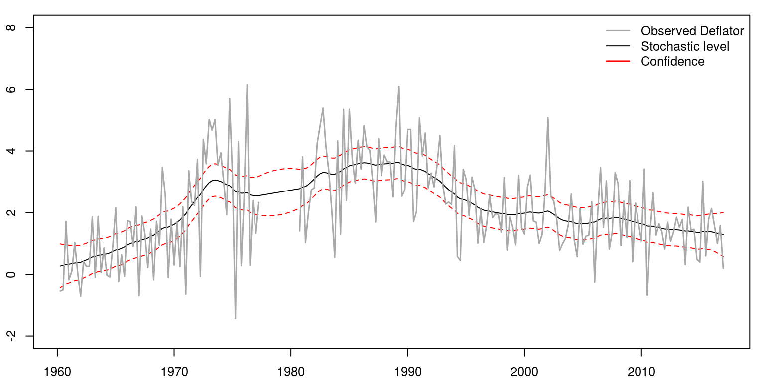
8 Regression effects with time-varying parameters
As utilised in class (and in the notes) we will consider the example that utilises data on the sale and price of spirits. This data file takes the form of a csv that has been labelled spirits.csv. To provide R with the location of the file, you can either provide the full extension for the csv file, or you can set the working directory with the aid of the setwd command. In what follows, I’ve used the second option, where we note that this file has information that pertains to two variables, spirits and price, which are stored as individual time series objects.
rm(list = ls())
graphics.off()

setwd("~/git/tsm/ts-4-tut/tut")

dat_tmp <- read.csv(file = "spirits.csv")
spirit <- ts(dat_tmp$spirit, start = c(1871, 1), end = c(1939,
    1), frequency = 1)
price <- ts(dat_tmp$price, start = c(1871, 1), end = c(1939,
    1), frequency = 1)
plot(ts.union(spirit, price), plot.type = "single")
We can then construct the model in much the same way as we did before, where in this case we are making use as price as an explanatory variable that is subject to a time-varying parameter.
fn <- function(parm) {
    mod <- dlmModPoly(order = 1) + dlmModReg(price, addInt = FALSE)
    V(mod) <- exp(parm[1])
    diag(W(mod))[1:2] <- exp(parm[2:3])
    return(mod)
}

fit <- dlmMLE(spirit, rep(0, 3), build = fn, hessian = TRUE)
conv <- fit$convergence  # zero for converged

loglik <- dlmLL(spirit, dlmModPoly(1) + dlmModReg(price,
    addInt = FALSE))

n.coef <- 3
r.aic <- (2 * (loglik)) + 2 * (sum(n.coef))  #dlmLL caculates the neg. LL
r.bic <- (2 * (loglik)) + (log(length(spirit))) * (n.coef)

mod <- fn(fit$par)
obs.error.var <- V(mod)
state.error.var <- diag(W(mod))

filtered <- dlmFilter(spirit, mod = mod)
smoothed <- dlmSmooth(filtered)
resids <- residuals(filtered, sd = FALSE)
mu <- dropFirst(smoothed$s[, 1])
betas <- dropFirst(smoothed$s[, 2])
mu.1 <- mu[1]
mu.end <- mu[length(mu)]
beta.1 <- betas[1]
beta.end <- betas[length(mu)]
8.1 Plotting the results
We can then display the results in much the same way as we did before, where we make use of three graphs that are displayed underneath one another.
par(mfrow = c(3, 1), mar = c(2.2, 2.2, 1, 1), cex = 0.8)
plot.ts(ts.union(spirit, mu), col = c("darkgrey", "black"),
    plot.type = "single", xlab = "", ylab = "", lwd = c(1.5,
        1))
legend("right", legend = c("Observed Deflator", "Stochastic level"),
    lwd = c(2, 1), col = c("darkgrey", "black"), bty = "n")

plot.ts(betas, col = "darkgrey", xlab = "", ylab = "", lwd = 1.5)
legend("topright", legend = "Coefficient", lwd = 1.5, col = "darkgrey",
    bty = "n")

plot.ts(resids, ylab = "", xlab = "", col = "darkgrey",
    lwd = 1.5)
abline(h = 0)
legend("topright", legend = "Residuals", lwd = 1.5, col = "darkgrey",
    bty = "n")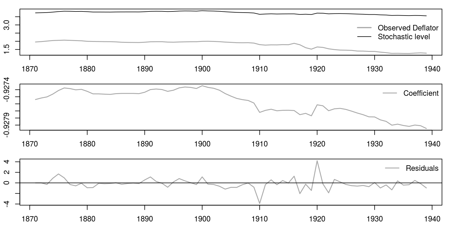
9 Multivariate state-space models
Unfortunately, when we want to work with multivariate models and where there are restrictions on some of the parameter matrices, we would need to make use of a matrix representation of the model. In what follows, we impose a number of restrictions on the convariance terms on one of the models to consider if the two time series variables are best described by a model that has a common trend. The example is contained in file T4-llmult.R and the data includes measures of economic output and prices. As was the case in the model with regression effects, we are going to read the data from csv file.
rm(list = ls())
graphics.off()

setwd("~/git/tsm/ts-4-tut/tut")

dat_tmp <- read.csv(file = "US_dat.csv")
dat <- ts(dat_tmp, start = c(1951, 1), frequency = 4)
plot.ts(dat)
To construct the model that does not have any restrictions on the covariance terms, we would proceed as follows:
build1 <- function(par) {
    m <- dlmModPoly(2)
    m$FF <- m$FF %x% diag(2)
    m$GG <- m$GG %x% diag(2)
    W1 <- diag(1e-07, nr = 2)
    W2 <- diag(exp(par[1:2]))
    W2[1, 2] <- W2[2, 1] <- tanh(par[3]) * prod(exp(0.5 *
        par[1:2]))
    m$W <- bdiag(W1, W2)
    V <- diag(exp(par[4:5]))
    V[1, 2] <- V[2, 1] <- tanh(par[6]) * prod(exp(0.5 *
        par[4:5]))
    m$V <- V
    m$m0 <- rep(0, 4)
    m$C0 <- diag(4) * 1e+07
    return(m)
}
We could then estimate the parameters and consider the model fit after calculating the Akaike information criteria.
mle <- vector("list", 2)
init <- cbind(as.matrix(expand.grid(rep(list(c(-3, 3)),
    4))), matrix(0, nc = 2, nr = 16))
init <- init[, c(1, 2, 5, 3, 4, 6)]
dimnames(init) <- NULL
for (i in 1:length(mle)) {
    mle[[i]] <- try(dlmMLE(dat, parm = init[i, ], build = build1,
        control = list(trace = 3, REPORT = 2)))
}
## N = 6, M = 5 machine precision = 2.22045e-16
## This problem is unconstrained.
## At X0, 0 variables are exactly at the bounds
## At iterate 0 f= -60.801 |proj g|= 52.231
## At iterate 2 f = -225.96 |proj g|= 34.653
## At iterate 4 f = -443.68 |proj g|= 49.049
## At iterate 6 f = -521.71 |proj g|= 34.451
## At iterate 8 f = -544.99 |proj g|= 10.35
## At iterate 10 f = -548.53 |proj g|= 2.1017
## At iterate 12 f = -548.95 |proj g|= 0.91642
## At iterate 14 f = -549.17 |proj g|= 0.84139
## At iterate 16 f = -549.2 |proj g|= 0.15497
## At iterate 18 f = -549.2 |proj g|= 0.12311
## At iterate 20 f = -549.21 |proj g|= 0.063508
## At iterate 22 f = -549.21 |proj g|= 0.0063328
## At iterate 24 f = -549.21 |proj g|= 0.0017712
##
## iterations 25
## function evaluations 33
## segments explored during Cauchy searches 1
## BFGS updates skipped 0
## active bounds at final generalized Cauchy point 0
## norm of the final projected gradient 0.00368313
## final function value -549.205
##
## F = -549.205
## final value -549.205206
## converged
## N = 6, M = 5 machine precision = 2.22045e-16
## This problem is unconstrained.
## At X0, 0 variables are exactly at the bounds
## At iterate 0 f= 136.61 |proj g|= 64.94
## At iterate 2 f = -537.33 |proj g|= 14.012
## At iterate 4 f = -542.16 |proj g|= 7.5494
## At iterate 6 f = -547.82 |proj g|= 6.0898
## At iterate 8 f = -548.89 |proj g|= 0.87905
## At iterate 10 f = -549.05 |proj g|= 0.90416
## At iterate 12 f = -549.19 |proj g|= 0.39742
## At iterate 14 f = -549.2 |proj g|= 0.1494
## At iterate 16 f = -549.21 |proj g|= 0.012187
## At iterate 18 f = -549.21 |proj g|= 0.012517
## At iterate 20 f = -549.21 |proj g|= 0.0040078
##
## iterations 21
## function evaluations 29
## segments explored during Cauchy searches 1
## BFGS updates skipped 0
## active bounds at final generalized Cauchy point 0
## norm of the final projected gradient 0.00398233
## final function value -549.205
##
## F = -549.205
## final value -549.205200
## convergedgood <- seq(along = mle)[sapply(mle, function(x) length(x) >
1 && x$conv == 0)]
mleX <- sapply(mle[good], function(x) unlist(x[1:2]))
mleX <- mleX[, order(mleX["value", ])]
fit1 <- build1(mleX[-NROW(mleX), 1])
loglik1 <- dlmLL(dat, fit1)
aic1 <- (2 * (loglik1)) + 2 * (sum(8)) #dlmLL caculates the neg. LLTo construct the model that has restricted covariance terms, we would proceed as follows:
build2 <- function(par) {
    m <- dlmModPoly(2)
    m$FF <- m$FF %x% diag(2)
    m$GG <- m$GG %x% diag(2)
    W1 <- diag(1e-07, nr = 2)
    W2 <- diag(exp(par[1:2]))
    # W2[1,2] <- W2[2,1] <- tanh(par[3]) * prod(exp(0.5 *
    # par[1 : 2]))
    m$W <- bdiag(W1, W2)
    V <- diag(exp(par[3:4]))
    V[1, 2] <- V[2, 1] <- tanh(par[5]) * prod(exp(0.5 *
        par[3:4]))
    m$V <- V
    m$m0 <- rep(0, 4)
    m$C0 <- diag(4) * 1e+07
    return(m)
}
We could then estimate the parameters and consider the model fit after calculating the Akaike information criteria.
mle <- vector("list", 2)
init <- cbind(as.matrix(expand.grid(rep(list(c(-3, 3)),
    4))), matrix(0, nc = 2, nr = 16))
init <- init[, c(1, 2, 4, 3, 5)]
dimnames(init) <- NULL
for (i in 1:length(mle)) {
    mle[[i]] <- try(dlmMLE(dat, parm = init[i, ], build = build2,
        control = list(trace = 3, REPORT = 2)))
}
## N = 5, M = 5 machine precision = 2.22045e-16
## This problem is unconstrained.
## At X0, 0 variables are exactly at the bounds
## At iterate 0 f= -60.801 |proj g|= 52.231
## At iterate 2 f = -225.96 |proj g|= 34.653
## At iterate 4 f = -443.64 |proj g|= 49.028
## At iterate 6 f = -519.61 |proj g|= 34.25
## At iterate 8 f = -541.92 |proj g|= 5.4749
## At iterate 10 f = -545.19 |proj g|= 5.5808
## At iterate 12 f = -546.59 |proj g|= 1.0118
## At iterate 14 f = -546.83 |proj g|= 0.17479
## At iterate 16 f = -546.84 |proj g|= 0.034
## At iterate 18 f = -546.84 |proj g|= 0.0046945
## At iterate 20 f = -546.84 |proj g|= 0.00053601
##
## iterations 20
## function evaluations 29
## segments explored during Cauchy searches 1
## BFGS updates skipped 0
## active bounds at final generalized Cauchy point 0
## norm of the final projected gradient 0.000536014
## final function value -546.84
##
## F = -546.84
## final value -546.839762
## converged
## N = 5, M = 5 machine precision = 2.22045e-16
## This problem is unconstrained.
## At X0, 0 variables are exactly at the bounds
## At iterate 0 f= 136.61 |proj g|= 64.94
## At iterate 2 f = -537.33 |proj g|= 14.014
## At iterate 4 f = -541.72 |proj g|= 5.2019
## At iterate 6 f = -546.13 |proj g|= 3.2787
## At iterate 8 f = -546.73 |proj g|= 0.98876
## At iterate 10 f = -546.83 |proj g|= 0.6204
## At iterate 12 f = -546.84 |proj g|= 0.0064185
## At iterate 14 f = -546.84 |proj g|= 0.0019832
##
## iterations 14
## function evaluations 21
## segments explored during Cauchy searches 1
## BFGS updates skipped 0
## active bounds at final generalized Cauchy point 0
## norm of the final projected gradient 0.00198323
## final function value -546.84
##
## F = -546.84
## final value -546.839761
## convergedgood <- seq(along = mle)[sapply(mle, function(x) length(x) >
1 && x$conv == 0)]
mleX <- sapply(mle[good], function(x) unlist(x[1:2]))
mleX <- mleX[, order(mleX["value", ])]
fit2 <- build2(mleX[-NROW(mleX), 1])
loglik2 <- dlmLL(dat, fit2)
aic2 <- (2 * (loglik2)) + 2 * (sum(6)) #dlmLL caculates the neg. LLTo compare the information criteria, we can look at the information criteria:
cat("Model 1 - AIC: ", aic1)## Model 1 - AIC: -1082.41cat("Model 2 - AIC: ", aic2)## Model 2 - AIC: -1081.68Since the information criteria for the first model is closer to negative infinity it provides a better fit of the data. We can then extract the results for the smoother as follows:
modelSmooth <- dlmSmooth(dat, mod = fit1)
Smooth.level.1 <- dropFirst(modelSmooth$s[, 1])
Smooth.level.2 <- dropFirst(modelSmooth$s[, 2])
Smooth.level.3 <- dropFirst(modelSmooth$s[, 3])
Smooth.level.4 <- dropFirst(modelSmooth$s[, 4])
To plot these results we can combine the data into separate objects before we invoke the plot command.
fig.1 <- ts.union(window(dat[, 1]), window(Smooth.level.1))

fig.2 <- ts.union(window(dat[, 2]), window(Smooth.level.2))

par(mfrow = c(2, 1), mar = c(2.2, 2.2, 1, 1), cex = 0.8)
plot(fig.1, plot.type = "single", col = c("blue", "green"),
    ylab = "")
legend("topright", legend = c("Inflation", "Smoothed"),
    lty = 1, col = c("blue", "green"), bty = "n")
plot(fig.2, plot.type = "single", col = c("blue", "green"),
    ylab = "")
legend("bottomright", legend = c("Ouput", "Smoothed"), lty = 1,
    col = c("blue", "green"), bty = "n")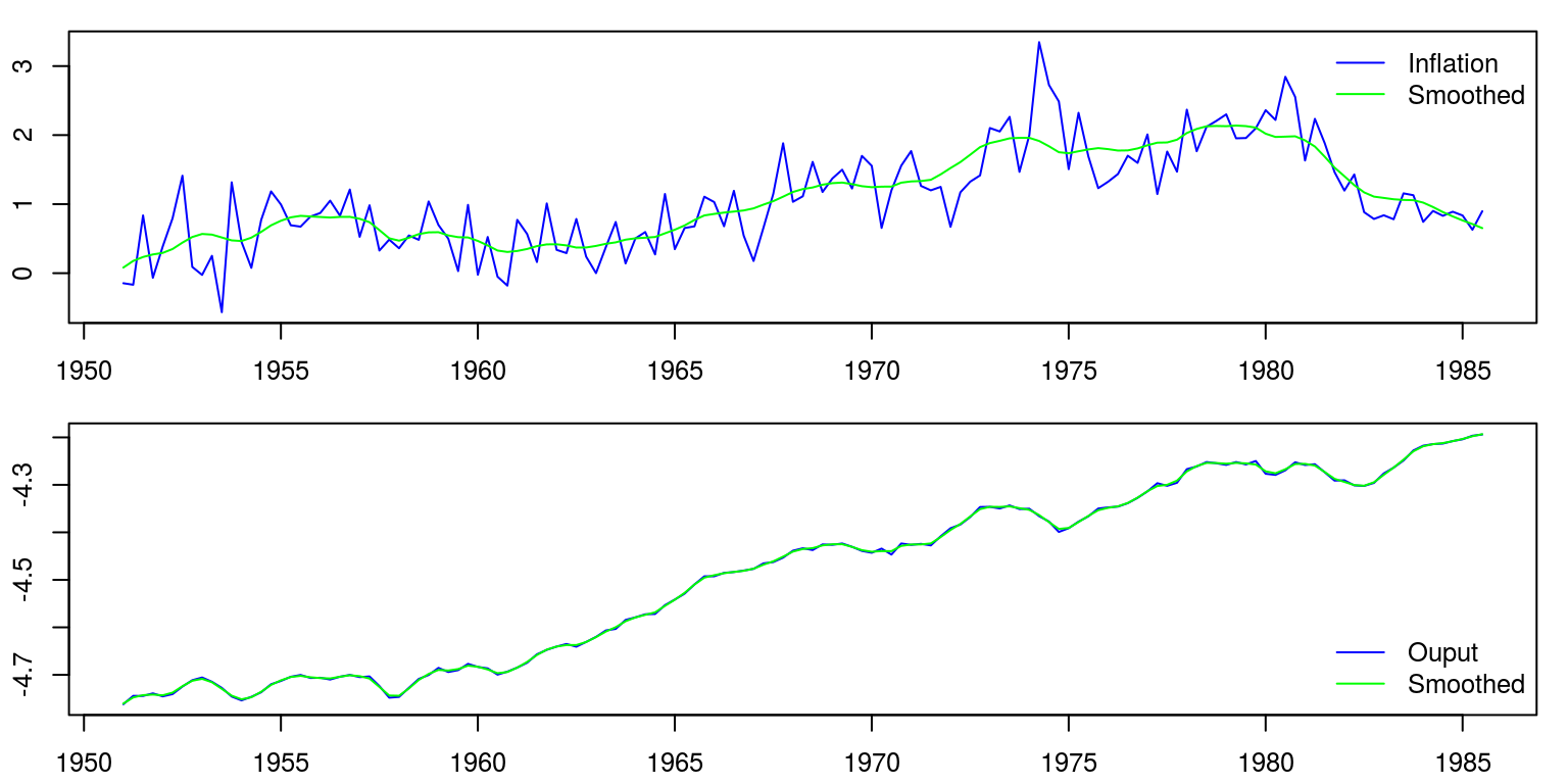
10 Coding the Kalman filter and smoother by hand
Of course one does not need to make use of packaged software routine to generate values for the Kalman filter and smoother. In the file sim_filter_smoother.R you will see how one could proceed through the respective steps to generate values for the unobserved variables. Note that everything is expressed with the aid of matrix algebra so the size of the coefficient and parameter matrices may increase as the model could incorporate a number of additional features.
You may wish to go through the respective steps of the filter and smoother, if you get a chance. The modelis currently set up to generate results for a local level model.
rm(list = ls())

set.seed(123456)
num <- 50  # simulate 50 observations

xi <- rnorm(num + 1, 0, 1)  # error in state equation
epsilon <- rnorm(num, 0, 1)  # error in measurement equation

alpha <- cumsum(xi)  # state equation takes form of random walk
yt <- alpha[-1] + epsilon  # obs: yt[1] ,..., yt[50]

## Objective now is to estimate values for alpha

# setup filter and smoother
alpha0 <- 0  # assume alpha_0 = N(0,1)
sigma0 <- 1  # assume alpha_0 = N(0,1)
Gt <- 1  # coefficient in state equation
Ft <- 1  # coefficient in measurement equation
cW <- 1  # state variance-covariance matrix
cV <- 1  # measurement variance-covariance matrix

## Kalman filter
W <- t(cW) %*% cW  # convert scalar to matrix
V <- t(cV) %*% cV  # convert scalar to matrix

Gt <- as.matrix(Gt)
pdim <- nrow(Gt)
yt <- as.matrix(yt)
qdim <- ncol(yt)
alphap <- array(NA, dim = c(pdim, 1, num))  # alpha_p= a_{t+1}
Pp <- array(NA, dim = c(pdim, pdim, num))  # Pp=P_{t+1}
alphaf <- array(NA, dim = c(pdim, 1, num))  # alpha_f=a_t
Pf <- array(NA, dim = c(pdim, pdim, num))  # Pf=P_t
innov <- array(NA, dim = c(qdim, 1, num))  # innovations
sig <- array(NA, dim = c(qdim, qdim, num))  # innov var-cov matrix
Kmat <- rep(NA, num)  # store Kalman gain

# initialize (because R can't count from zero)
alpha00 <- as.matrix(alpha0, nrow = pdim, ncol = 1)  # state: mean starting value
P00 <- as.matrix(sigma0, nrow = pdim, ncol = pdim)  # state: variance start value
alphap[, , 1] <- Gt %*% alpha00  # predicted value a_{t+1}
Pp[, , 1] <- Gt %*% P00 %*% t(Gt) + W  # variance for predicted state value
sigtemp <- Ft %*% Pp[, , 1] %*% t(Ft) + V  # variance for measurement value
sig[, , 1] <- (t(sigtemp) + sigtemp)/2  # innov var - make sure it's symmetric
siginv <- solve(sig[, , 1])  # 1 / innov var
K <- Pp[, , 1] %*% t(Ft) %*% siginv  # K_t = predicted variance / innov variance
Kmat[1] <- K  # store Kalman gain
innov[, , 1] <- yt[1, ] - Ft %*% alphap[, , 1]  # epsilon_t = y_t - a_t
alphaf[, , 1] <- alphap[, , 1] + K %*% innov[, , 1]  # a_{t+1} = a_t + K_t(epsilon_t)
Pf[, , 1] <- Pp[, , 1] - K %*% Ft %*% Pp[, , 1]  # variance of forecast
sigmat <- as.matrix(sig[, , 1], nrow = qdim, ncol = qdim)  # collect variance of measurement errors
like <- log(det(sigmat)) + t(innov[, , 1]) %*% siginv %*%
    innov[, , 1]  # calculate -log(likelihood)

########## start filter iterations ###################
for (i in 2:num) {
    if (num < 2)
        break
    alphap[, , i] <- Gt %*% alphaf[, , i - 1]  # predicted value a_{t+2}
    Pp[, , i] <- Gt %*% Pf[, , i - 1] %*% t(Gt) + W  # variance of predicted state estimate
    sigtemp <- Ft %*% Pp[, , i] %*% t(Ft) + V  # variance of measurement error
    sig[, , i] <- (t(sigtemp) + sigtemp)/2  # innov var - make sure it's symmetric
    siginv <- solve(sig[, , i])
    K <- Pp[, , i] %*% t(Ft) %*% siginv  # K_t = predicted variance / innov variance
    Kmat[i] <- K  # store Kalman gain
    innov[, , i] <- yt[i, ] - Ft %*% alphap[, , i]  # epsilon_t = y_t - a_t
    alphaf[, , i] <- alphap[, , i] + K %*% innov[, , i]  # a_{t+1} = a_t + K_t(epsilon_t)
    Pf[, , i] <- Pp[, , i] - K %*% Ft %*% Pp[, , i]  # variance of forecast
    sigmat <- as.matrix(sig[, , i], nrow = qdim, ncol = qdim)  # collect variance of measurement errors
    like <- like + log(det(sigmat)) + t(innov[, , i]) %*%
        siginv %*% innov[, , i]  # calculate -log(likelihood)
}
like <- 0.5 * like

kf <- list(alphap = alphap, Pp = Pp, alphaf = alphaf, Pf = Pf,
    like = like, innov = innov, sig = sig, Kn = K)

## Kalman smoother
pdim <- nrow(as.matrix(Gt))
alphas <- array(NA, dim = c(pdim, 1, num))  # alpha_s = smoothed alpha values
Ps <- array(NA, dim = c(pdim, pdim, num))  # Ps=P_t^s
J <- array(NA, dim = c(pdim, pdim, num))  # J=J_t
alphas[, , num] <- kf$alphaf[, , num]  # starting value for a_T^s
Ps[, , num] <- kf$Pf[, , num]  # starting value for prediction variance

########## start smoother iterations ###################
for (k in num:2) {
    J[, , k - 1] <- (kf$Pf[, , k - 1] %*% t(Gt)) %*% solve(kf$Pp[,
        , k])
    alphas[, , k - 1] <- kf$alphaf[, , k - 1] + J[, , k -
        1] %*% (alphas[, , k] - kf$alphap[, , k])
    Ps[, , k - 1] <- kf$Pf[, , k - 1] + J[, , k - 1] %*%
        (Ps[, , k] - kf$Pp[, , k]) %*% t(J[, , k - 1])
}
# and now for the initial values because R can't count
# backward to zero
alpha00 <- alpha0
P00 <- sigma0
J0 <- as.matrix((P00 %*% t(Gt)) %*% solve(kf$Pp[, , 1]),
    nrow = pdim, ncol = pdim)
alpha0n <- as.matrix(alpha00 + J0 %*% (alphas[, , 1] - kf$alphap[,
    , 1]), nrow = pdim, ncol = 1)
P0n <- P00 + J0 %*% (Ps[, , k] - kf$Pp[, , k]) %*% t(J0)

ks <- list(alphas = alphas, Ps = Ps, alpha0n = alpha0n,
    P0n = P0n, J0 = J0, J = J, alphap = kf$alphap, Pp = kf$Pp,
    alphaf = kf$alphaf, Pf = kf$Pf, like = kf$like, Kn = kf$K)
To plot the results, we are then able to proceed as follows:
par(mfrow = c(3, 1), mar = c(2, 5, 2, 1))
Time <- 1:num
plot(Time, alpha[-1], main = "Prediction", ylim = c(-5,
    20), xlab = "", ylab = "")
lines(ks$alphap)
lines(ks$alphap + 2 * sqrt(ks$Pp), lty = "dashed", col = "blue")
lines(ks$alphap - 2 * sqrt(ks$Pp), lty = "dashed", col = "blue")
plot(Time, alpha[-1], main = "Filter", ylim = c(-5, 20),
    xlab = "", ylab = "")
lines(ks$alphaf)
lines(ks$alphaf + 2 * sqrt(ks$Pf), lty = "dashed", col = "blue")
lines(ks$alphaf - 2 * sqrt(ks$Pf), lty = "dashed", col = "blue")
plot(Time, alpha[-1], main = "Smoother", ylim = c(-5, 20),
    xlab = "", ylab = "")
lines(ks$alphas)
lines(ks$alphas + 2 * sqrt(ks$Ps), lty = "dashed", col = "blue")
lines(ks$alphas - 2 * sqrt(ks$Ps), lty = "dashed", col = "blue")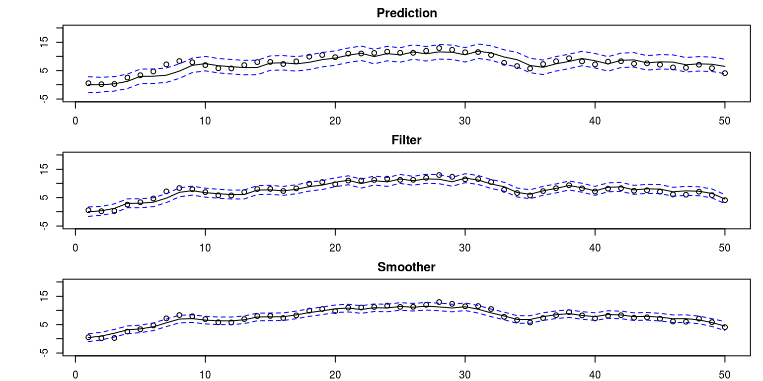
pred.error <- ks$alphap[1, 1, ] - ks$alphaf[1, 1, ]
par(mfrow = c(2, 1), mar = c(2, 2, 2, 1), cex = 0.65)
plot(Kmat, main = "Kalman Gain", xlab = "", ylab = "")
plot(pred.error, main = "Prediction Errors", xlab = "",
    ylab = "", type = "l")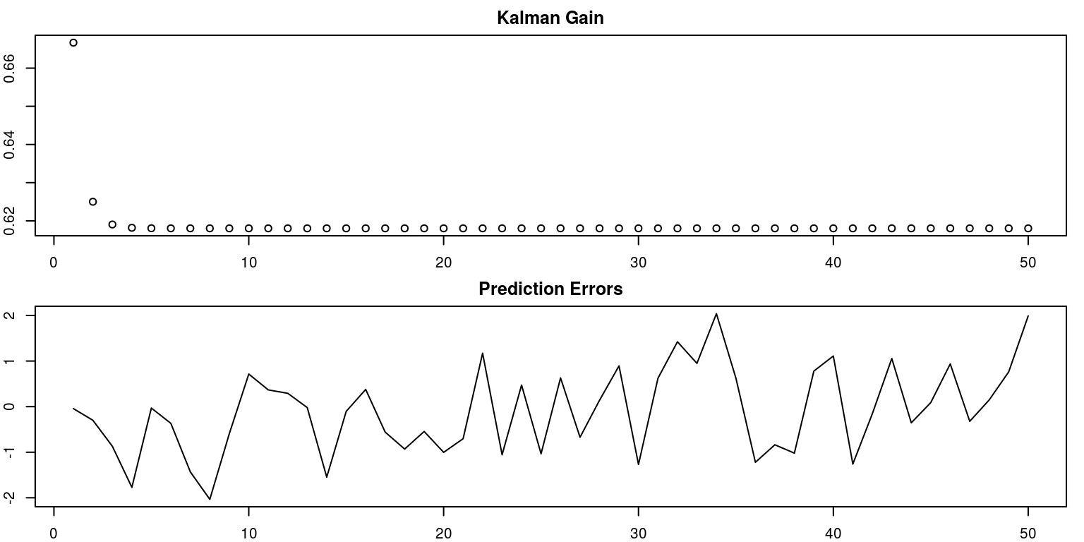
To consider the model diagnostics we can look at the preiction errors, with the aid of the following commands.
ac(pred.error)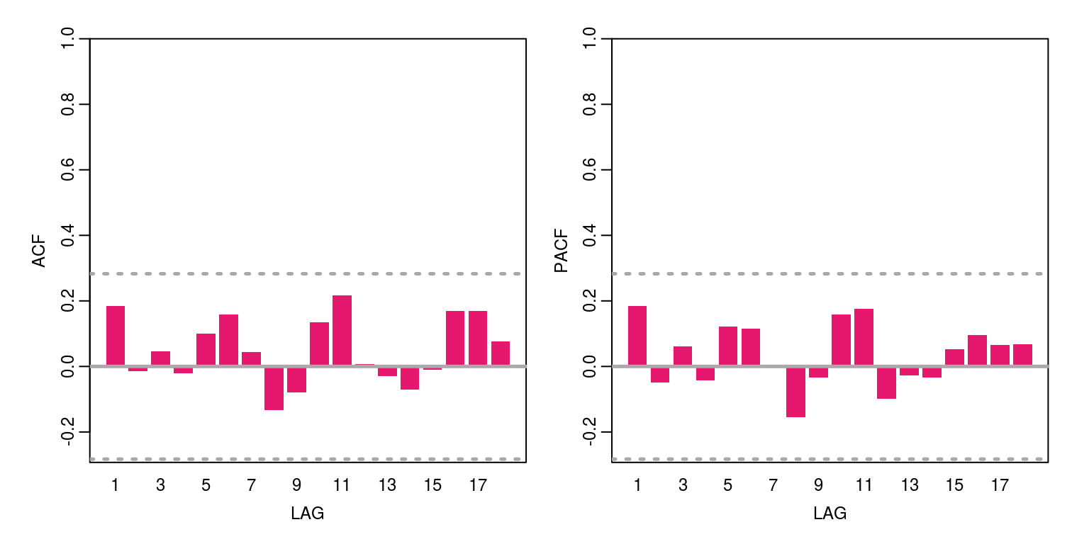
par(mfrow = c(1, 1), mar = c(2, 5, 2, 1))
hist(pred.error, main = "")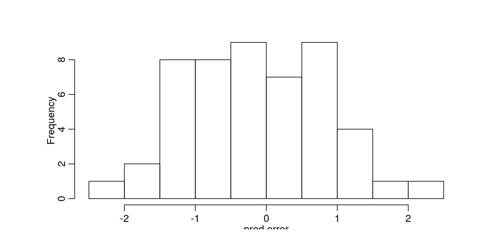
alpha[1]## [1] 0.8337332ks$alpha0n## [,1]
## [1,] 0.206708sqrt(ks$P0n) # initial value info## [,1]
## [1,] 0.8342936