Tutorial: Nonstationarity
by Kevin Kotzé
1 Implementing the Dickey-Fuller Test
The first exercise makes use of the Dickey-Fuller test that is applied to simulated data. This example is contained in the file T6-URtest.R, where we look to simulate a number of stationary and nonstationary time series that are then subjected to the one-sided test that imposes the null of a unit root.
Once again, the first thing that we do is clear all variables from the current environment and close all the plots. This is performed with the following commands:
rm(list = ls())
graphics.off()
Thereafter, we will need to install the tsm package from my GitHub account, as well as the vars package that containts a number of unit root tests.
devtools::install_github("KevinKotze/tsm")
install.packages("vars")
The next step is to make sure that you can access the routines in these packages by making use of the library command.
library(tsm)
library(vars)
1.1 Simulate the data
Prior to generating the data we set the seed so that we get similar results. To then generate values for a pure random walk, rw, we just sum a sequency of white noise errors (i.e. the effects of shocks do not dissipate). The time trend, trd, is a sequence of observations than spans from 1 to 500 and the random walk with drift includes the realisations for the random walk and the deterministic time trend. The trend stationary process, dt, includes just the deterministic trend and noise and an ar1 process with a coefficient of 0.8 is simulated with the aid of the arima.sim command.
set.seed(123456)
e <- rnorm(500)
rw <- cumsum(e)
trd <- 1:500
rw.wd <- 0.5 * trd + cumsum(e)
dt <- e + 0.5 * trd
ar1 <- arima.sim(model = list(ar = 0.8), n = 500)
To ensure that these calculations have been performed correctly, we could inspect the data with the plot.ts command.
plot.ts(rw)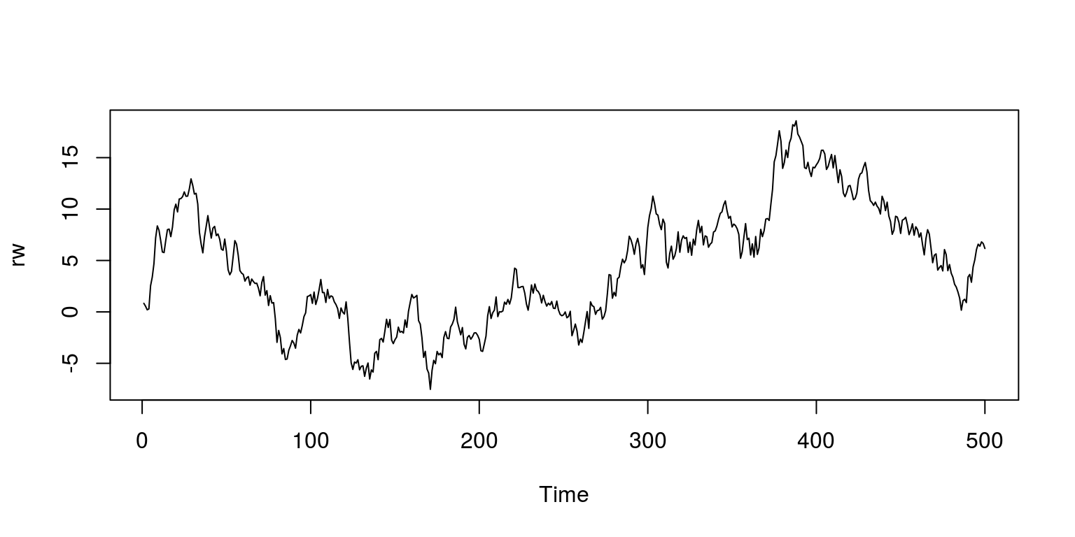
1.2 Using the Dickey-Fuller test
To test the null hypothesis that the time series variables contain a unit root, we may apply the augmented Dickey-Fuller test. This procedure is contained in the vars package and is executed with the ur.df command. When using this command the number of lags of the dependent variable in the test equation could be determined by information criteria. In what follows we have used the Akaike Information Criteria to determine the lag length. To determine which of the three different test equations will be ustilised, we need to specify the deterministic aspects that need to be included, which may be none (for no deterministic elements), drift (for a constant in the test equation) or trend (for both a constant and a time trend).
By way of example, we test the random walk for a unit root in what follows using the three different test equations. In this case, we follow the practice of moving from the general to the specific test equations:
rw.ct <- ur.df(rw, type = "trend", selectlags = c("AIC"))
summary(rw.ct)
##
## ###############################################
## # Augmented Dickey-Fuller Test Unit Root Test #
## ###############################################
##
## Test regression trend
##
##
## Call:
## lm(formula = z.diff ~ z.lag.1 + 1 + tt + z.diff.lag)
##
## Residuals:
## Min 1Q Median 3Q Max
## -3.7020 -0.6573 0.0375 0.6871 2.7374
##
## Coefficients:
## Estimate Std. Error t value Pr(>|t|)
## (Intercept) 0.0179687 0.0897702 0.200 0.8414
## z.lag.1 -0.0198456 0.0089144 -2.226 0.0264 *
## tt 0.0003226 0.0003532 0.914 0.3614
## z.diff.lag 0.0268074 0.0449937 0.596 0.5516
## ---
## Signif. codes:
## 0 '***' 0.001 '**' 0.01 '*' 0.05 '.' 0.1 ' ' 1
##
## Residual standard error: 0.9967 on 494 degrees of freedom
## Multiple R-squared: 0.01027, Adjusted R-squared: 0.004257
## F-statistic: 1.708 on 3 and 494 DF, p-value: 0.1644
##
##
## Value of test-statistic is: -2.2262 1.6816 2.4917
##
## Critical values for test statistics:
## 1pct 5pct 10pct
## tau3 -3.98 -3.42 -3.13
## phi2 6.15 4.71 4.05
## phi3 8.34 6.30 5.36rw.t <- ur.df(rw, type = "drift", selectlags = c("AIC"))
summary(rw.t)##
## ###############################################
## # Augmented Dickey-Fuller Test Unit Root Test #
## ###############################################
##
## Test regression drift
##
##
## Call:
## lm(formula = z.diff ~ z.lag.1 + 1 + z.diff.lag)
##
## Residuals:
## Min 1Q Median 3Q Max
## -3.6998 -0.6682 0.0229 0.6927 2.7514
##
## Coefficients:
## Estimate Std. Error t value Pr(>|t|)
## (Intercept) 0.081673 0.056529 1.445 0.1491
## z.lag.1 -0.015973 0.007841 -2.037 0.0422 *
## z.diff.lag 0.024681 0.044926 0.549 0.5830
## ---
## Signif. codes:
## 0 '***' 0.001 '**' 0.01 '*' 0.05 '.' 0.1 ' ' 1
##
## Residual standard error: 0.9965 on 495 degrees of freedom
## Multiple R-squared: 0.008595, Adjusted R-squared: 0.004589
## F-statistic: 2.146 on 2 and 495 DF, p-value: 0.1181
##
##
## Value of test-statistic is: -2.0372 2.1057
##
## Critical values for test statistics:
## 1pct 5pct 10pct
## tau2 -3.44 -2.87 -2.57
## phi1 6.47 4.61 3.79rw.none <- ur.df(rw, type = "none", selectlags = c("AIC"))
summary(rw.none)##
## ###############################################
## # Augmented Dickey-Fuller Test Unit Root Test #
## ###############################################
##
## Test regression none
##
##
## Call:
## lm(formula = z.diff ~ z.lag.1 - 1 + z.diff.lag)
##
## Residuals:
## Min 1Q Median 3Q Max
## -3.6791 -0.6218 0.0913 0.7350 2.7544
##
## Coefficients:
## Estimate Std. Error t value Pr(>|t|)
## z.lag.1 -0.009027 0.006201 -1.456 0.146
## z.diff.lag 0.021860 0.044933 0.487 0.627
##
## Residual standard error: 0.9976 on 496 degrees of freedom
## Multiple R-squared: 0.004541, Adjusted R-squared: 0.0005269
## F-statistic: 1.131 on 2 and 496 DF, p-value: 0.3235
##
##
## Value of test-statistic is: -1.4558
##
## Critical values for test statistics:
## 1pct 5pct 10pct
## tau1 -2.58 -1.95 -1.62To interpret the results of the first test equation, note that the values of the test statistics are -2.2262, 1.6816, 2.4917. The first of these pertains to the value of \(\pi\) and since it is not less than the critical value of tau3 we are unable to reject the null of a unit root. The values of the other test statistics pertain to the F-tests, which suggest that the deterministic elements should be removed from the test equations as they do not exceed the critical values for phi2 and phi3.
When utilising a general to specific framework, the results of previous regression suggest that one would need to drop the deterministic time trained period. Therefore, the second test equation makes use of the test equation with only a constant. As would be expected, the F-test suggests that the constant should be dropped. The final test then excludes all deterministic elements and one is unable to reject the null that the variable contains a unit root as the test statistic of -1.4558 is not smaller than the critical values.
If we concluded that the variable does not contain a unit root, as one would be able to do for the AR(1) model, one could inspect the residual for remaining serial correlation. This would involve plotting the residuals with the plot.ts command and making use of an autocorrelation function.
plot.ts(rw.none@res, ylab = "Residuals")
abline(h = 0, col = "red")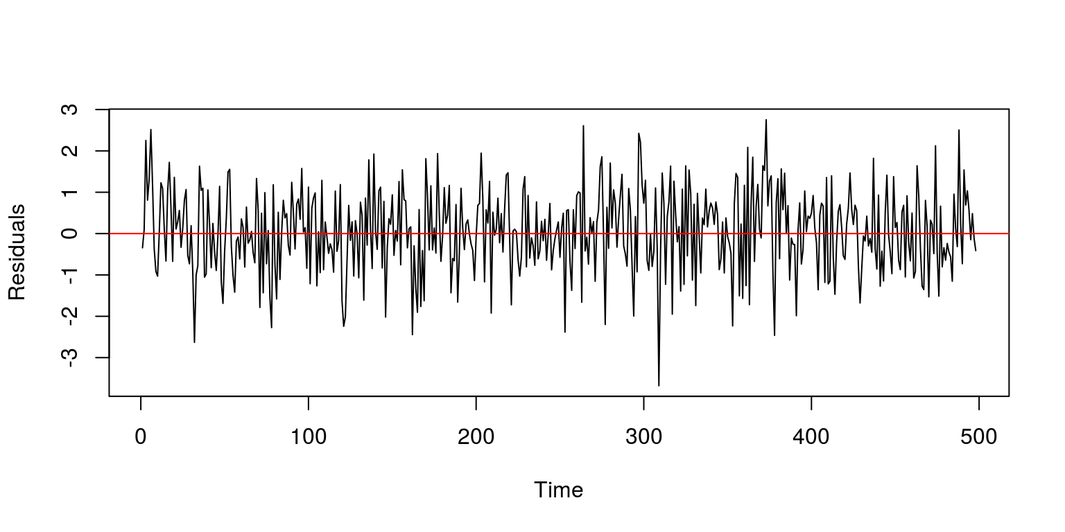
ac(rw.none@res, max.lag = 20)
As an alternative to the above procedure, where we test all of the three test equations individually, we could make use of the gts_ur command, which executes the three test equations in a sequential manner, moving from the general-to-specific functional form.
gts_ur(rw)##
## #################
## ## ADF summary ##
## #################
##
## Cannot reject null of unit root at 5% - no deterministic
##
## ## ADF with constrant and time trend ##
## statistic 1pct 5pct 10pct
## pi -2.23 -3.98 -3.42 -3.13
## varphi3 1.68 6.15 4.71 4.05
## varphi3 2.49 8.34 6.30 5.36
##
## Cannot reject null of unit root at 5%
## Cannot reject null of no trend at 5%
## Cannot reject null of no constant and no trend at 5%
##
## ## ADF with constrant ##
## statistic 1pct 5pct 10pct
## pi -2.04 -3.44 -2.87 -2.57
## varphi1 2.11 6.47 4.61 3.79
##
## Cannot reject null of unit root at 5%
## Cannot reject null of no constant at 5%
##
## ## ADF with no deterministic ##
## statistic 1pct 5pct 10pct
## pi -1.46 -2.58 -1.95 -1.62
##
## Cannot reject null of unit root at 5%
## In this case the notation that has been used follows that of the notes for this section.
A similar procedure could be used to test the null of a unit root in a similar variable. In this case we conclude that the appropriate test equation contains a constant for the drift and we are unable to reject the null of a unit root.
rwd.ct <- ur.df(rw.wd, type = "trend", selectlags = c("AIC"))
summary(rwd.ct)
##
## ###############################################
## # Augmented Dickey-Fuller Test Unit Root Test #
## ###############################################
##
## Test regression trend
##
##
## Call:
## lm(formula = z.diff ~ z.lag.1 + 1 + tt + z.diff.lag)
##
## Residuals:
## Min 1Q Median 3Q Max
## -3.7020 -0.6573 0.0375 0.6871 2.7374
##
## Coefficients:
## Estimate Std. Error t value Pr(>|t|)
## (Intercept) 0.504565 0.092826 5.436 8.6e-08 ***
## z.lag.1 -0.019846 0.008914 -2.226 0.0264 *
## tt 0.010245 0.004636 2.210 0.0275 *
## z.diff.lag 0.026807 0.044994 0.596 0.5516
## ---
## Signif. codes:
## 0 '***' 0.001 '**' 0.01 '*' 0.05 '.' 0.1 ' ' 1
##
## Residual standard error: 0.9967 on 494 degrees of freedom
## Multiple R-squared: 0.01027, Adjusted R-squared: 0.004257
## F-statistic: 1.708 on 3 and 494 DF, p-value: 0.1644
##
##
## Value of test-statistic is: -2.2262 35.0913 2.4917
##
## Critical values for test statistics:
## 1pct 5pct 10pct
## tau3 -3.98 -3.42 -3.13
## phi2 6.15 4.71 4.05
## phi3 8.34 6.30 5.36rwd.t <- ur.df(rw.wd, type = "drift", selectlags = c("AIC"))
summary(rwd.t)##
## ###############################################
## # Augmented Dickey-Fuller Test Unit Root Test #
## ###############################################
##
## Test regression drift
##
##
## Call:
## lm(formula = z.diff ~ z.lag.1 + 1 + z.diff.lag)
##
## Residuals:
## Min 1Q Median 3Q Max
## -3.7635 -0.6669 0.0348 0.6928 2.6561
##
## Coefficients:
## Estimate Std. Error t value Pr(>|t|)
## (Intercept) 0.5269428 0.0926340 5.688 2.2e-08 ***
## z.lag.1 -0.0001874 0.0005998 -0.312 0.755
## z.diff.lag 0.0168499 0.0449429 0.375 0.708
## ---
## Signif. codes:
## 0 '***' 0.001 '**' 0.01 '*' 0.05 '.' 0.1 ' ' 1
##
## Residual standard error: 1.001 on 495 degrees of freedom
## Multiple R-squared: 0.00048, Adjusted R-squared: -0.003558
## F-statistic: 0.1189 on 2 and 495 DF, p-value: 0.888
##
##
## Value of test-statistic is: -0.3125 49.8037
##
## Critical values for test statistics:
## 1pct 5pct 10pct
## tau2 -3.44 -2.87 -2.57
## phi1 6.47 4.61 3.79par(mfrow = c(1, 1), mar = c(4.2, 4.2, 2, 1), cex = 0.8)
plot.ts(rwd.t@res, ylab = "Residuals")
abline(h = 0, col = "red")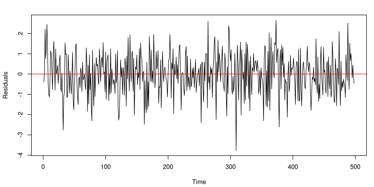
ac(rwd.t@res, max.lag = 20)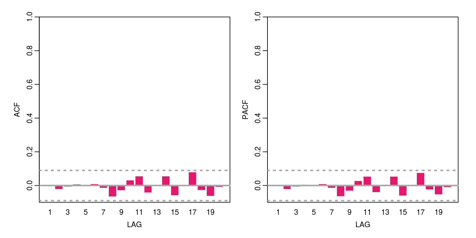
gts_ur(rw.wd)##
## #################
## ## ADF summary ##
## #################
##
## Unable to reject null of unit root at 5% - with constant & trend
##
## ## ADF with constrant and time trend ##
## statistic 1pct 5pct 10pct
## pi -2.23 -3.98 -3.42 -3.13
## varphi3 35.09 6.15 4.71 4.05
## varphi3 2.49 8.34 6.30 5.36
##
## Cannot reject null of unit root at 5%
## Cannot reject null of no trend at 5%
## Able to reject null of no constant and no trend at 5%
##
## ## ADF with constrant ##
## statistic 1pct 5pct 10pct
## pi -0.31 -3.44 -2.87 -2.57
## varphi1 49.80 6.47 4.61 3.79
##
## Cannot reject null of unit root at 5%
## Able to reject null of no constant at 5%
##
## ## ADF with no deterministic ##
## statistic 1pct 5pct 10pct
## pi 7.95 -2.58 -1.95 -1.62
##
## Cannot reject null of unit root at 5%
## 2 Dornbusch Overshooting
In what follows we make use of real world data to apply the Dickey-Fuller test. In this case we have data for the real exchange rate and we would like to test which shocks to the exchange rate have a permanent effect. The exercise is contained in the T6_REER.R example. Hence, we proceed as we have done on many occasions previously.
rm(list = ls())
graphics.off()
As we will now need to make use of data that is contained in a CSV file, we are going to need to set the working directory.
setwd("~/git/tsm/ts-6-tut")
# setwd('C:\\Users\\image')
To access the routines that are contained in the vars and tsm packages, we make use of the following library commands.
library(vars)
library(tsm)
We are then able to read the CSV file before we create the time series variables for each of the respective real exchange rates. Note that this data is measured at a quarterly frequency.
dat <- read.csv(file = "reer.csv")
aus <- ts(dat$Australia, start = c(1980, 1), frequency = 4)
can <- ts(dat$Canada, start = c(1980, 1), frequency = 4)
fra <- ts(dat$France, start = c(1980, 1), frequency = 4)
ger <- ts(dat$Germany, start = c(1980, 1), frequency = 4)
uk <- ts(dat$UK, start = c(1980, 1), frequency = 4)
us <- ts(dat$US, start = c(1980, 1), frequency = 4)
To ensure that we have completed the above tasks correctly we plot some of the data on a graph with the following commands.
plot(cbind(uk, us, ger), plot.type = "single", col = c("blue",
    "green", "red"), ylab = "")
legend("bottomright", legend = c("uk", "us", "ger"), lty = 1,
    col = c("blue", "green", "red"), bty = "n")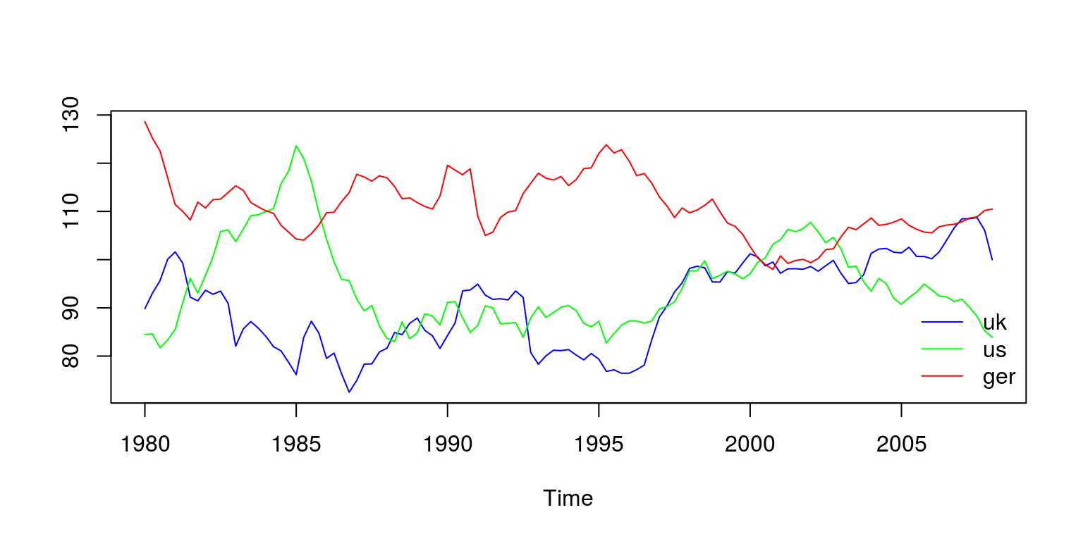
Note that each of these time series seems to meander like a random walk and there is little evidence of explosive behaviour or deterministic time trends. To consider the degree of persistence in the data make use of the autocorrelation function, which suggests that all of the data is highly persistent.
ac(uk, max.lag = 20)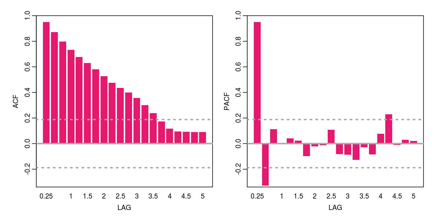
ac(us, max.lag = 20)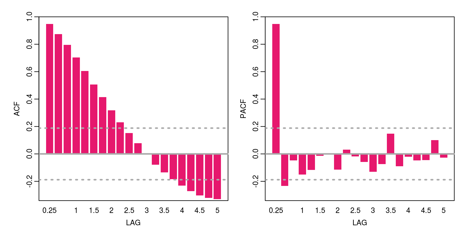
ac(ger, max.lag = 20)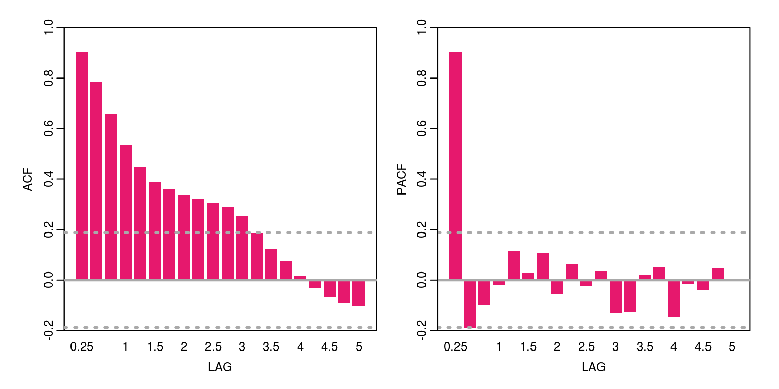
To test for unit roots we can then make use of the Dickey-Fuller test. Note that in this case the underlying theory of purchasing power parity would not allow for the inclusion of a deterministic time trend. However, the test equation may include a constant.
dfc.ger <- ur.df(log(ger), type = "drift", selectlags = c("AIC"))
summary(dfc.ger)
##
## ###############################################
## # Augmented Dickey-Fuller Test Unit Root Test #
## ###############################################
##
## Test regression drift
##
##
## Call:
## lm(formula = z.diff ~ z.lag.1 + 1 + z.diff.lag)
##
## Residuals:
## Min 1Q Median 3Q Max
## -0.08296 -0.01121 -0.00062 0.01039 0.04944
##
## Coefficients:
## Estimate Std. Error t value Pr(>|t|)
## (Intercept) 0.43608 0.14237 3.063 0.002767 **
## z.lag.1 -0.09279 0.03025 -3.068 0.002726 **
## z.diff.lag 0.34983 0.08660 4.039 0.000101 ***
## ---
## Signif. codes:
## 0 '***' 0.001 '**' 0.01 '*' 0.05 '.' 0.1 ' ' 1
##
## Residual standard error: 0.01729 on 108 degrees of freedom
## Multiple R-squared: 0.1816, Adjusted R-squared: 0.1664
## F-statistic: 11.98 on 2 and 108 DF, p-value: 2e-05
##
##
## Value of test-statistic is: -3.0678 4.7877
##
## Critical values for test statistics:
## 1pct 5pct 10pct
## tau2 -3.46 -2.88 -2.57
## phi1 6.52 4.63 3.81plot(dfc.ger)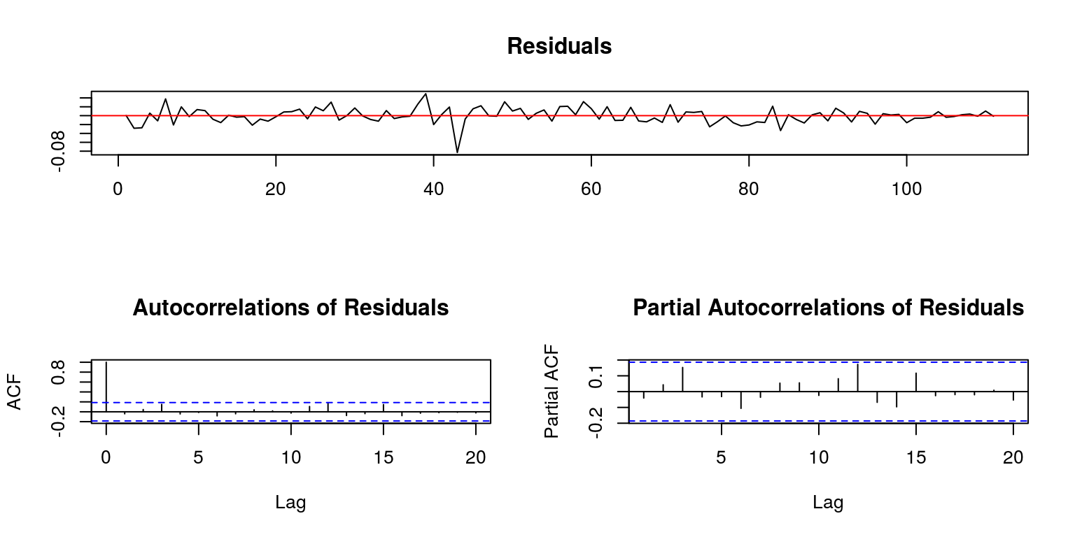
The results of this test suggest that we are able to reject null of unit root.
dfc.aus <- ur.df(log(aus), type = "drift", selectlags = c("AIC"))
summary(dfc.aus)
##
## ###############################################
## # Augmented Dickey-Fuller Test Unit Root Test #
## ###############################################
##
## Test regression drift
##
##
## Call:
## lm(formula = z.diff ~ z.lag.1 + 1 + z.diff.lag)
##
## Residuals:
## Min 1Q Median 3Q Max
## -0.147577 -0.017398 0.006226 0.020216 0.076510
##
## Coefficients:
## Estimate Std. Error t value Pr(>|t|)
## (Intercept) 0.23653 0.13813 1.712 0.0897 .
## z.lag.1 -0.04959 0.02898 -1.711 0.0899 .
## z.diff.lag 0.13311 0.09567 1.391 0.1670
## ---
## Signif. codes:
## 0 '***' 0.001 '**' 0.01 '*' 0.05 '.' 0.1 ' ' 1
##
## Residual standard error: 0.03724 on 108 degrees of freedom
## Multiple R-squared: 0.03739, Adjusted R-squared: 0.01956
## F-statistic: 2.097 on 2 and 108 DF, p-value: 0.1278
##
##
## Value of test-statistic is: -1.711 1.4666
##
## Critical values for test statistics:
## 1pct 5pct 10pct
## tau2 -3.46 -2.88 -2.57
## phi1 6.52 4.63 3.81plot(dfc.aus)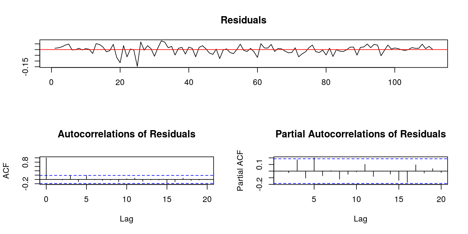
dfc.aus <- ur.df(log(aus), type = "none", selectlags = c("AIC"))
summary(dfc.aus)
##
## ###############################################
## # Augmented Dickey-Fuller Test Unit Root Test #
## ###############################################
##
## Test regression none
##
##
## Call:
## lm(formula = z.diff ~ z.lag.1 - 1 + z.diff.lag)
##
## Residuals:
## Min 1Q Median 3Q Max
## -0.145921 -0.014099 0.005538 0.021264 0.081677
##
## Coefficients:
## Estimate Std. Error t value Pr(>|t|)
## z.lag.1 0.0000236 0.0007482 0.032 0.975
## z.diff.lag 0.1062619 0.0952072 1.116 0.267
##
## Residual standard error: 0.03757 on 109 degrees of freedom
## Multiple R-squared: 0.01132, Adjusted R-squared: -0.00682
## F-statistic: 0.6241 on 2 and 109 DF, p-value: 0.5377
##
##
## Value of test-statistic is: 0.0315
##
## Critical values for test statistics:
## 1pct 5pct 10pct
## tau1 -2.58 -1.95 -1.62plot(dfc.aus)
For the case of Australia, we cannot reject null of unit root
dfc.can <- ur.df(log(can), type = "drift", selectlags = c("AIC"))
summary(dfc.can)
##
## ###############################################
## # Augmented Dickey-Fuller Test Unit Root Test #
## ###############################################
##
## Test regression drift
##
##
## Call:
## lm(formula = z.diff ~ z.lag.1 + 1 + z.diff.lag)
##
## Residuals:
## Min 1Q Median 3Q Max
## -0.046902 -0.018403 -0.000975 0.016340 0.070304
##
## Coefficients:
## Estimate Std. Error t value Pr(>|t|)
## (Intercept) 0.13128 0.09521 1.379 0.17081
## z.lag.1 -0.02736 0.02000 -1.368 0.17412
## z.diff.lag 0.33432 0.09284 3.601 0.00048 ***
## ---
## Signif. codes:
## 0 '***' 0.001 '**' 0.01 '*' 0.05 '.' 0.1 ' ' 1
##
## Residual standard error: 0.0234 on 108 degrees of freedom
## Multiple R-squared: 0.1115, Adjusted R-squared: 0.09508
## F-statistic: 6.779 on 2 and 108 DF, p-value: 0.001685
##
##
## Value of test-statistic is: -1.3681 1.0474
##
## Critical values for test statistics:
## 1pct 5pct 10pct
## tau2 -3.46 -2.88 -2.57
## phi1 6.52 4.63 3.81plot(dfc.can)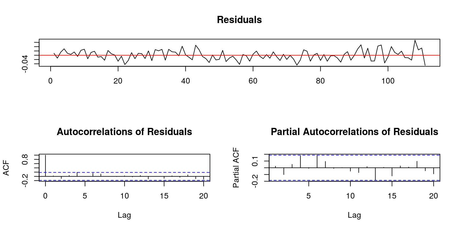
dfc.can <- ur.df(log(can), type = "none", selectlags = c("AIC"))
summary(dfc.can)
##
## ###############################################
## # Augmented Dickey-Fuller Test Unit Root Test #
## ###############################################
##
## Test regression none
##
##
## Call:
## lm(formula = z.diff ~ z.lag.1 - 1 + z.diff.lag)
##
## Residuals:
## Min 1Q Median 3Q Max
## -0.051226 -0.017995 -0.000786 0.016245 0.068495
##
## Coefficients:
## Estimate Std. Error t value Pr(>|t|)
## z.lag.1 0.0002059 0.0004697 0.438 0.66200
## z.diff.lag 0.3128275 0.0918987 3.404 0.00093 ***
## ---
## Signif. codes:
## 0 '***' 0.001 '**' 0.01 '*' 0.05 '.' 0.1 ' ' 1
##
## Residual standard error: 0.02349 on 109 degrees of freedom
## Multiple R-squared: 0.09982, Adjusted R-squared: 0.0833
## F-statistic: 6.043 on 2 and 109 DF, p-value: 0.003243
##
##
## Value of test-statistic is: 0.4383
##
## Critical values for test statistics:
## 1pct 5pct 10pct
## tau1 -2.58 -1.95 -1.62plot(dfc.can)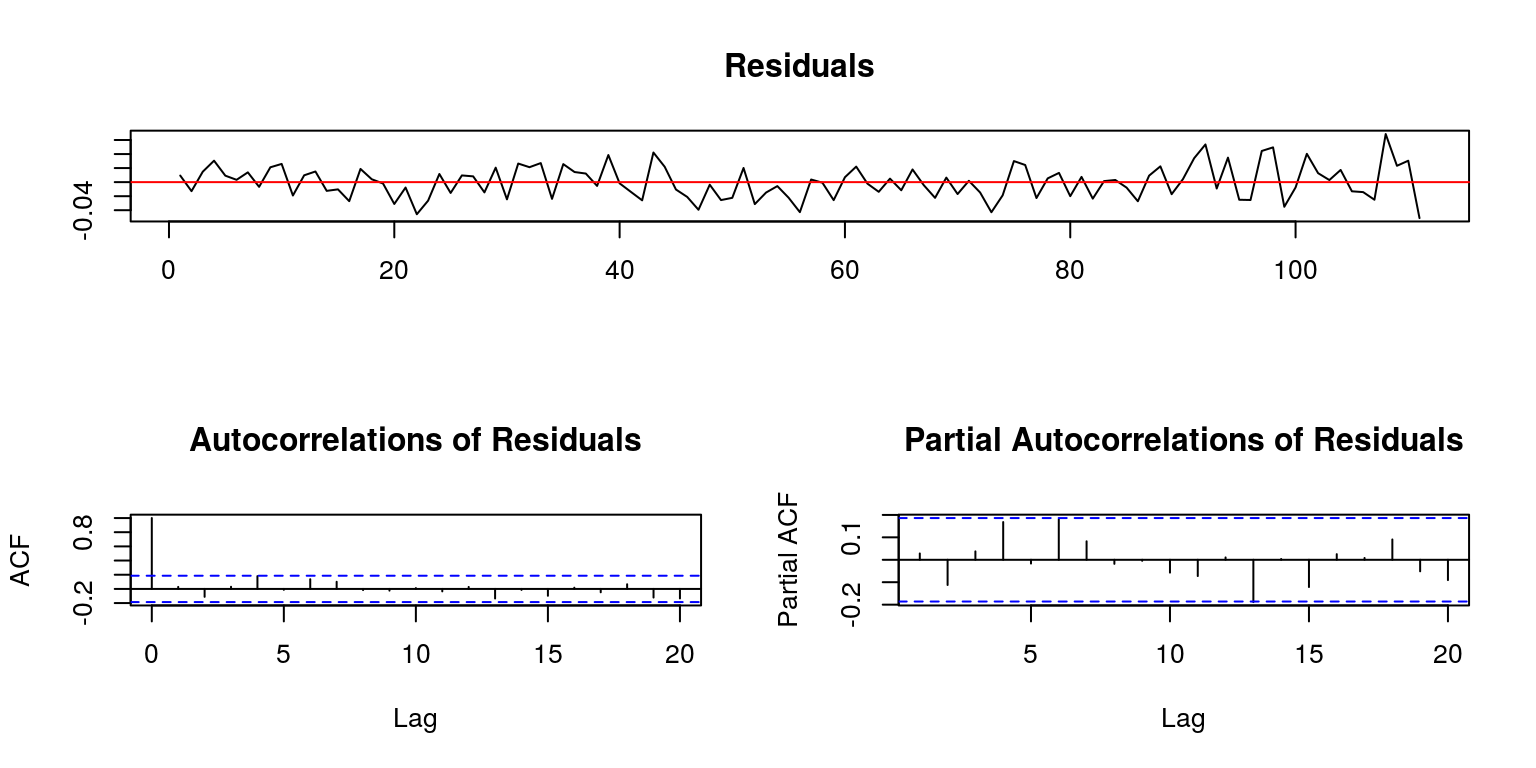
Similarly so for Canada and for France.
dfc.fra <- ur.df(log(fra), type = "drift", selectlags = c("AIC"))
summary(dfc.fra)
##
## ###############################################
## # Augmented Dickey-Fuller Test Unit Root Test #
## ###############################################
##
## Test regression drift
##
##
## Call:
## lm(formula = z.diff ~ z.lag.1 + 1 + z.diff.lag)
##
## Residuals:
## Min 1Q Median 3Q Max
## -0.063992 -0.007148 0.001282 0.008559 0.031415
##
## Coefficients:
## Estimate Std. Error t value Pr(>|t|)
## (Intercept) 0.41639 0.14718 2.829 0.00556 **
## z.lag.1 -0.08903 0.03143 -2.832 0.00551 **
## z.diff.lag 0.24486 0.09134 2.681 0.00850 **
## ---
## Signif. codes:
## 0 '***' 0.001 '**' 0.01 '*' 0.05 '.' 0.1 ' ' 1
##
## Residual standard error: 0.01429 on 108 degrees of freedom
## Multiple R-squared: 0.1126, Adjusted R-squared: 0.09619
## F-statistic: 6.853 on 2 and 108 DF, p-value: 0.001577
##
##
## Value of test-statistic is: -2.8324 4.0677
##
## Critical values for test statistics:
## 1pct 5pct 10pct
## tau2 -3.46 -2.88 -2.57
## phi1 6.52 4.63 3.81plot(dfc.fra)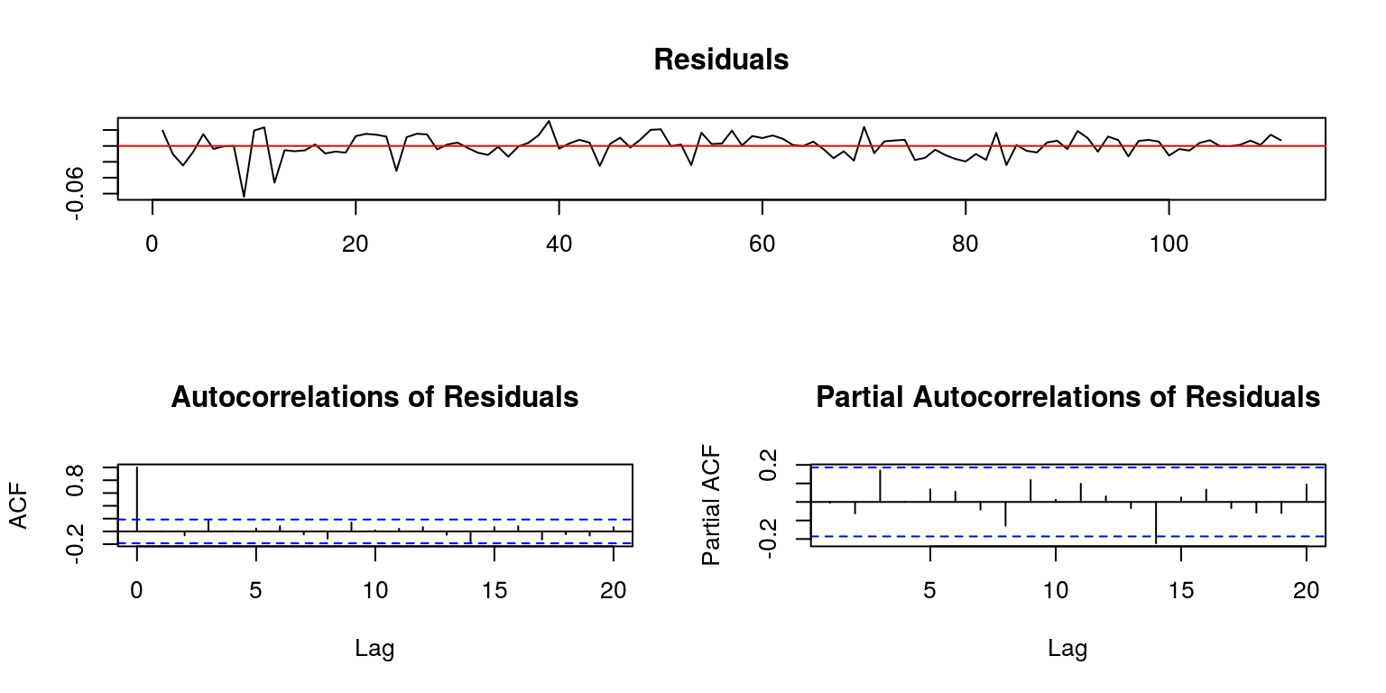
dfc.fra <- ur.df(log(fra), type = "none", selectlags = c("AIC"))
summary(dfc.fra)
##
## ###############################################
## # Augmented Dickey-Fuller Test Unit Root Test #
## ###############################################
##
## Test regression none
##
##
## Call:
## lm(formula = z.diff ~ z.lag.1 - 1 + z.diff.lag)
##
## Residuals:
## Min 1Q Median 3Q Max
## -0.065968 -0.005841 0.000366 0.008296 0.032620
##
## Coefficients:
## Estimate Std. Error t value Pr(>|t|)
## z.lag.1 -0.0001050 0.0002992 -0.351 0.7263
## z.diff.lag 0.2163626 0.0936494 2.310 0.0228 *
## ---
## Signif. codes:
## 0 '***' 0.001 '**' 0.01 '*' 0.05 '.' 0.1 ' ' 1
##
## Residual standard error: 0.01475 on 109 degrees of freedom
## Multiple R-squared: 0.0484, Adjusted R-squared: 0.03094
## F-statistic: 2.772 on 2 and 109 DF, p-value: 0.06695
##
##
## Value of test-statistic is: -0.351
##
## Critical values for test statistics:
## 1pct 5pct 10pct
## tau1 -2.58 -1.95 -1.62plot(dfc.fra)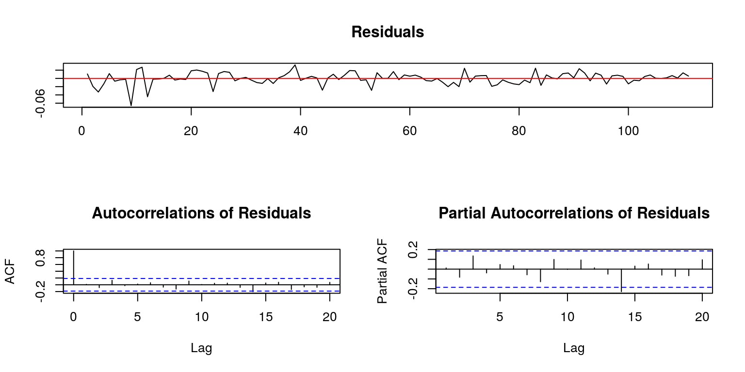
3 Unit root tests when the data includes a structural break
In this case we use simulated data to consider how a structural break may influence the test statistics that are used to identify a unit root. In addition, we also make use of the Zivot & Andrews test to consider the use of unit root tests that allow for an endogenous structural break. This exercise is contained in the T6_strucbreak.R file.
rm(list = ls())
graphics.off()

library(vars)
library(tsm)
The simulated data is initially constructed as before:
set.seed(123456)
e <- rnorm(500)
rw <- cumsum(e)
trd <- 1:500
rw.wd <- 0.5 * trd + cumsum(e)
dt <- e + 0.5 * trd
ar1 <- arima.sim(list(order = c(1, 0, 0), ar = 0.7), n = 500)
To introduce a structural break at observation 250 we construct a dummy.
S <- c(rep(0, 249), rep(1, 251))We then create three variables that incorporate a large structural break and different degrees of persistence. These variables are then plotted with the plot.ts command.
y.st <- 15 * S + rw
x.st <- ar1 + 15 * S
e.st <- e + 15 * S

plot.ts(cbind(y.st, x.st, e.st), main = "")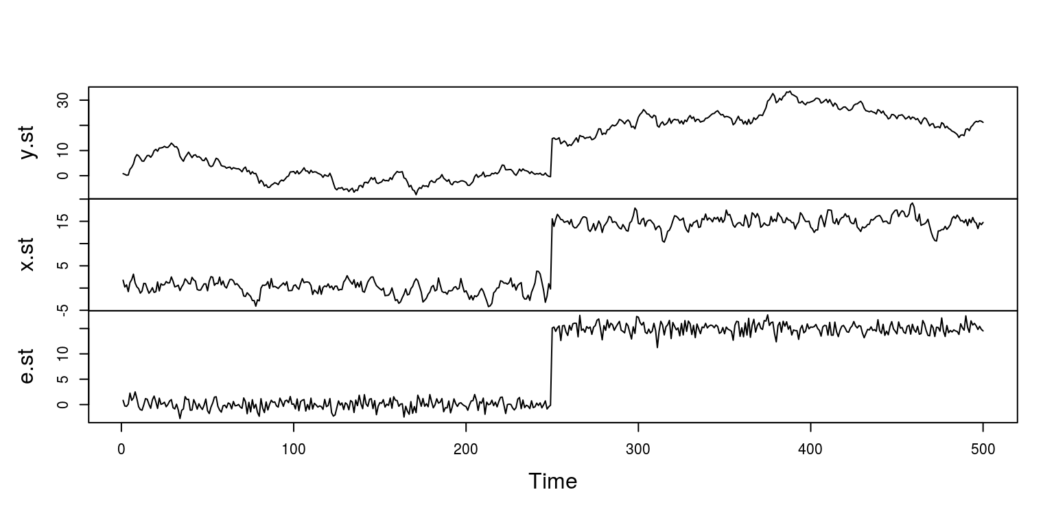
The first test that we will run is for the white noise with a structural break.
gts_ur(e.st)##
## #################
## ## ADF summary ##
## #################
##
## Cannot reject null of unit root at 5% - no deterministic
##
## ## ADF with constrant and time trend ##
## statistic 1pct 5pct 10pct
## pi -3.01 -3.98 -3.42 -3.13
## varphi3 3.16 6.15 4.71 4.05
## varphi3 4.54 8.34 6.30 5.36
##
## Cannot reject null of unit root at 5%
## Cannot reject null of no trend at 5%
## Cannot reject null of no constant and no trend at 5%
##
## ## ADF with constrant ##
## statistic 1pct 5pct 10pct
## pi -1.56 -3.44 -2.87 -2.57
## varphi1 1.41 6.47 4.61 3.79
##
## Cannot reject null of unit root at 5%
## Cannot reject null of no constant at 5%
##
## ## ADF with no deterministic ##
## statistic 1pct 5pct 10pct
## pi -0.66 -2.58 -1.95 -1.62
##
## Cannot reject null of unit root at 5%
## Note that in this case we are unable to reject the null of a unit root. This is relatively problematic. To remove the structural break one could regress the variable on the dummy and then test the residuals for the presence of a unit root.
resids <- (lm(e.st ~ S - 1))$residuals
est.n <- ur.df(resids, type = "none", selectlags = c("AIC"))
summary(est.n)
##
## ###############################################
## # Augmented Dickey-Fuller Test Unit Root Test #
## ###############################################
##
## Test regression none
##
##
## Call:
## lm(formula = z.diff ~ z.lag.1 - 1 + z.diff.lag)
##
## Residuals:
## Min 1Q Median 3Q Max
## -3.7628 -0.6616 0.0417 0.6802 2.6618
##
## Coefficients:
## Estimate Std. Error t value Pr(>|t|)
## z.lag.1 -1.00483 0.06297 -15.958 <2e-16 ***
## z.diff.lag 0.02178 0.04487 0.485 0.628
## ---
## Signif. codes:
## 0 '***' 0.001 '**' 0.01 '*' 0.05 '.' 0.1 ' ' 1
##
## Residual standard error: 0.9993 on 496 degrees of freedom
## Multiple R-squared: 0.4919, Adjusted R-squared: 0.4898
## F-statistic: 240 on 2 and 496 DF, p-value: < 2.2e-16
##
##
## Value of test-statistic is: -15.958
##
## Critical values for test statistics:
## 1pct 5pct 10pct
## tau1 -2.58 -1.95 -1.62In this case one is able to reject the null of a unit root.
3.1 Endogenous structural breaks
When we are unsure as to whether or not there is a structural break in the data, or if we are unsure as to the exact location of the structural break, we make use of the Zivot & Andrews test. This may be implemented with the ur.za command.
za.est <- ur.za(e.st, model = "both", lag = 0)  # white noise
summary(za.est)
##
## ################################
## # Zivot-Andrews Unit Root Test #
## ################################
##
##
## Call:
## lm(formula = testmat)
##
## Residuals:
## Min 1Q Median 3Q Max
## -3.8472 -0.6542 0.0418 0.6866 2.6369
##
## Coefficients:
## Estimate Std. Error t value Pr(>|t|)
## (Intercept) 0.0154105 0.1282259 0.120 0.904
## y.l1 0.0106659 0.0371717 0.287 0.774
## trend -0.0001615 0.0008875 -0.182 0.856
## du 15.0082235 0.5830535 25.741 <2e-16 ***
## dt -0.0007670 0.0012442 -0.616 0.538
## ---
## Signif. codes:
## 0 '***' 0.001 '**' 0.01 '*' 0.05 '.' 0.1 ' ' 1
##
## Residual standard error: 1.001 on 494 degrees of freedom
## (1 observation deleted due to missingness)
## Multiple R-squared: 0.9828, Adjusted R-squared: 0.9826
## F-statistic: 7039 on 4 and 494 DF, p-value: < 2.2e-16
##
##
## Teststatistic: -26.6153
## Critical values: 0.01= -5.57 0.05= -5.08 0.1= -4.82
##
## Potential break point at position: 249plot(za.est)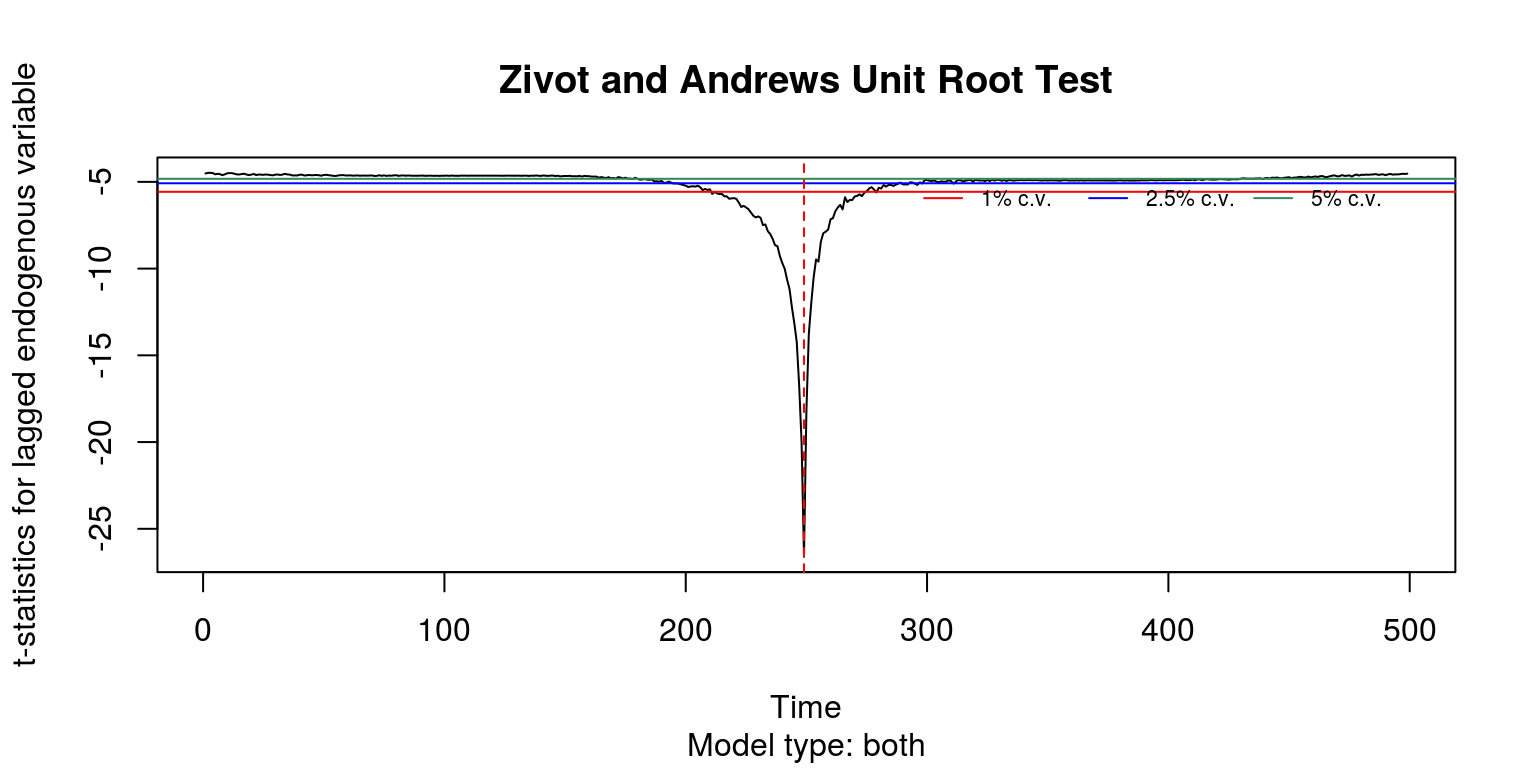
Note that in this case we reject the null of a unit root as the test stastic has a value of -21.63 and the critical value (at 5%) is -5.08. In addition, it is evident from the plot that the proposed structural break in the middle of the sample, clearly cuts through all the confidence intervals.
4 Testing the null hypothesis of stationarity
As an alternative to the Dickey-Fuller test, one could employ the KPSS approach, which tests the null of stationarity. This exercise is contained in the T6_KPSS.R file. To consider an example with simulated data, we could proceed as follows:
rm(list = ls())
graphics.off()

library(vars)set.seed(123456)
e <- rnorm(500)
rw <- cumsum(e)
trd <- 1:500
rw.wd <- 0.5 * trd + cumsum(e)
dt <- e + 0.5 * trdThe command to use the KPSS test is then ur.kpss and the test equations include variants for the alternative hypothesis. These pertain to cases of difference stationary mu and trend stationary tau. The lags can be set to none, short or long.
set.seed(123456)
e <- rnorm(500)
rw <- cumsum(e)
trd <- 1:500
rw.wd <- 0.5 * trd + cumsum(e)
dt <- e + 0.5 * trdWhen testing the time series for white noise, we note that we are unable to reject null of stationarity, against the alternative of difference stationarity.
e.kpss <- ur.kpss(e, type = "mu", use.lag = NULL)
summary(e.kpss)
##
## #######################
## # KPSS Unit Root Test #
## #######################
##
## Test is of type: mu with 5 lags.
##
## Value of test-statistic is: 0.0564
##
## Critical value for a significance level of:
## 10pct 5pct 2.5pct 1pct
## critical values 0.347 0.463 0.574 0.739However, when applying this test to the random walk we note that we are able to reject the null of stationarity against the alternative of difference and trend stationarity.
rw.kpss <- ur.kpss(rw, type = "mu", use.lag = NULL)
summary(rw.kpss)
##
## #######################
## # KPSS Unit Root Test #
## #######################
##
## Test is of type: mu with 5 lags.
##
## Value of test-statistic is: 3.2172
##
## Critical value for a significance level of:
## 10pct 5pct 2.5pct 1pct
## critical values 0.347 0.463 0.574 0.739rw.kpss <- ur.kpss(rw, type = "tau", use.lag = NULL)
summary(rw.kpss)##
## #######################
## # KPSS Unit Root Test #
## #######################
##
## Test is of type: tau with 5 lags.
##
## Value of test-statistic is: 0.9467
##
## Critical value for a significance level of:
## 10pct 5pct 2.5pct 1pct
## critical values 0.119 0.146 0.176 0.2165 Applying these test to inflation data
To apply these tests to year-on-year inflation data for South Africa we make use of the data that has been incorporated in the tsm package. This exercise is contained in the T6_inf.R file.
rm(list = ls())
graphics.off()

library(vars)
library(tsm)
To load the data and create time series object we proceed as before:
dat <- sarb_month$KBP7170N
cpi <- ts(na.omit(dat), start = c(2002, 1), frequency = 12)
inf <- diff(cpi, lag = 12)/cpi[-1 * (length(cpi) - 11):length(cpi)]

plot(inf)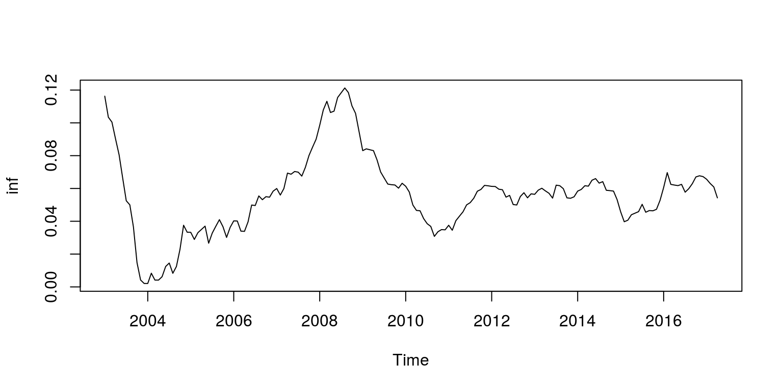
We can then perform the Dickey-Fuller test, where we note that we are unable to reject null of non-stationarity.
gts_ur(inf)##
## #################
## ## ADF summary ##
## #################
##
## Cannot reject null of unit root at 5% - no deterministic
##
## ## ADF with constrant and time trend ##
## statistic 1pct 5pct 10pct
## pi -2.71 -3.99 -3.43 -3.13
## varphi3 2.61 6.22 4.75 4.07
## varphi3 3.82 8.43 6.49 5.47
##
## Cannot reject null of unit root at 5%
## Cannot reject null of no trend at 5%
## Cannot reject null of no constant and no trend at 5%
##
## ## ADF with constrant ##
## statistic 1pct 5pct 10pct
## pi -2.56 -3.46 -2.88 -2.57
## varphi1 3.37 6.52 4.63 3.81
##
## Cannot reject null of unit root at 5%
## Cannot reject null of no constant at 5%
##
## ## ADF with no deterministic ##
## statistic 1pct 5pct 10pct
## pi -1.38 -2.58 -1.95 -1.62
##
## Cannot reject null of unit root at 5%
## When we perform the Zivot & Andrews test we note that there would appear to be a structural break in the data, at observation 71, and that when we account for this we are able to reject the null of a unit root.
za.inf <- ur.za(inf, model = "both", lag = 1)
summary(za.inf)
##
## ################################
## # Zivot-Andrews Unit Root Test #
## ################################
##
##
## Call:
## lm(formula = testmat)
##
## Residuals:
## Min 1Q Median 3Q Max
## -0.0147649 -0.0026897 0.0004672 0.0025394 0.0118238
##
## Coefficients:
## Estimate Std. Error t value Pr(>|t|)
## (Intercept) -1.956e-03 1.164e-03 -1.680 0.094926 .
## y.l1 9.014e-01 1.772e-02 50.879 < 2e-16 ***
## trend 1.975e-04 3.537e-05 5.584 9.57e-08 ***
## y.dl1 2.538e-01 6.991e-02 3.630 0.000379 ***
## du -7.537e-03 1.573e-03 -4.792 3.68e-06 ***
## dt -1.835e-04 3.792e-05 -4.838 3.01e-06 ***
## ---
## Signif. codes:
## 0 '***' 0.001 '**' 0.01 '*' 0.05 '.' 0.1 ' ' 1
##
## Residual standard error: 0.004291 on 164 degrees of freedom
## (2 observations deleted due to missingness)
## Multiple R-squared: 0.9675, Adjusted R-squared: 0.9665
## F-statistic: 976.8 on 5 and 164 DF, p-value: < 2.2e-16
##
##
## Teststatistic: -5.5632
## Critical values: 0.01= -5.57 0.05= -5.08 0.1= -4.82
##
## Potential break point at position: 71plot(za.inf)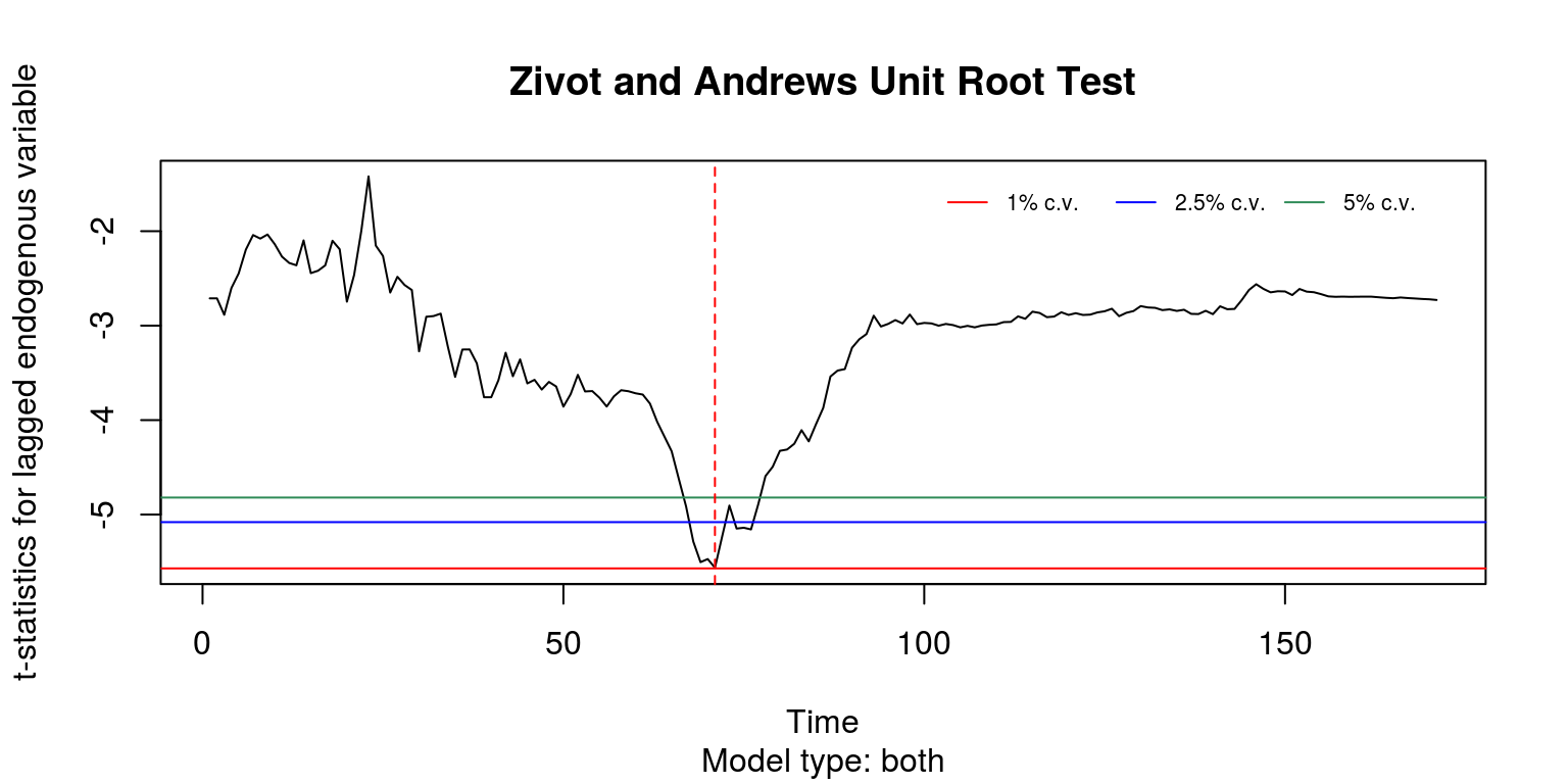
To obtain the date for observation 71, we can use the command:
time(inf)[71]## [1] 2008.833which coincides with the date of the Global Financial Crisis. In addition, when we make use of the KPSS test we note that we are unable to reject the null of stationarity, since the test statistic is smaller than the critical value.
kpss.inf <- ur.kpss(inf, type = "mu", use.lag = NULL)
summary(kpss.inf)
##
## #######################
## # KPSS Unit Root Test #
## #######################
##
## Test is of type: mu with 4 lags.
##
## Value of test-statistic is: 0.2975
##
## Critical value for a significance level of:
## 10pct 5pct 2.5pct 1pct
## critical values 0.347 0.463 0.574 0.7396 Simulaton for bias and power studies
In the final part of the tutorial, we consider the inherent bias that is contained in the estimation of the coefficients in a unit root process, by employing a simulation procedure. Thereafter, we make use of a power study to consider the probability of being unable to reject a false null hypothesis.
6.1 The estimation bias in a unit root model
After opening up the file T6_DickeyFuller.R, we once again clear everything to start afresh.
rm(list = ls())
graphics.off()
We then set the seed before we specify the number of observations in the time series, noo, the coefficient value for the AR(1) regression, phi, and the number of simulations that need to be performed, nos. The coefficient estimates are then going to be stored in the vector phi_mat.
set.seed(123456)
noo <- 100
phi <- 1
nos <- 10000

phi_mat <- rep(0, nos)
To execute the study we make use of a loop, where we simulate values for the time seres variable where the coefficient estimate is given, and then try to re-estimate this coefficient for the given data.
for (i in 1:nos) {
    y <- filter(rnorm(noo), filter = phi, method = "recursive")
    x <- y[-noo]
    y <- y[-1]
    phiest <- (lm(y ~ x - 1))$coef
    phi_mat[i] <- phiest
}

hist(phi_mat, 50, main = "", xlab = "")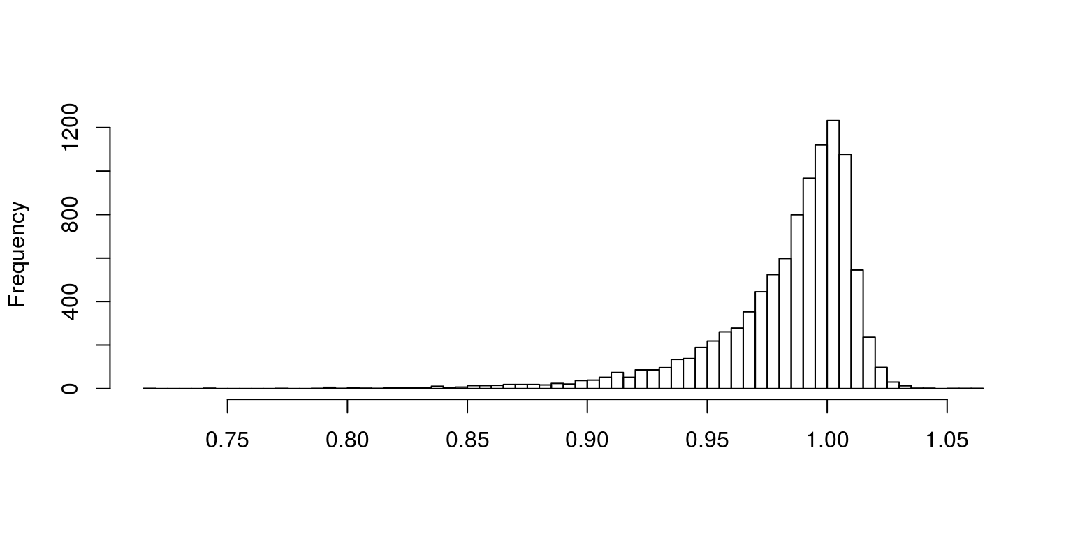
The plot of the coefficients shows that the estimates are skewed to be below the value of one on many occasions. And the mean bias could be calculated as:
mean(phi_mat - phi)## [1] -0.01708207which would always be less than zero.
6.2 Power studies for the Dickey-Fuller test
It has been noted that the Dickey-Fuller test may suggest that a stationary time series (which is fairly persistent) may contain a unit root. To consider the probability of this occuring we conduct a similar simulation exercise for an AR(1) process that has a coefficient of 0.95. We then calculate the number of times that we are able to reject the null of a unit root at the different critical levels. The code for such a study is contained in the T6_DFpower.R file and it would look something like this:
rm(list = ls())
graphics.off()set.seed(123456)
noo <- 100
phi <- 0.95
nos <- 10000
phi_mat <- rep(0, nos)
tvalue <- rep(0, nos)
for (i in 1:nos) {
y <- filter(rnorm(noo), filter = phi, method = "recursive")
x <- y[-noo]
y <- y[-1]
phiest <- (lm(y ~ x - 1))$coef
phi_mat[i] <- phiest
sig <- sum((y - phiest * x)^2)/(noo - 1)
var <- sig * solve(Conj(t(x)) %*% x)
tvalue[i] <- (phiest - phi)/sqrt(var)
}
terror1 <- rep(0, nos)
for (i in 1:nos) {
if (tvalue[i] < -2.5866)
terror1[i] <- 1
}
terror2 <- rep(0, nos)
for (i in 1:nos) {
if (tvalue[i] < -1.9433)
terror2[i] <- 1
}
terror3 <- rep(0, nos)
for (i in 1:nos) {
if (tvalue[i] < -1.6174)
terror3[i] <- 1
}
cat("AR(1) coefficient = ", phi, "\n")## AR(1) coefficient = 0.95cat("rejection probability at 1% = ", mean(terror1), "\n")## rejection probability at 1% = 0.0081Using critical values for the 1% level of significance, we reject the false null hypothesis less than 1% of the time.
cat("rejection probability at 5% = ", mean(terror2), "\n")## rejection probability at 5% = 0.0428And when using critical values for the 5% level of significance, we reject the false null hypothesis less than 5% of the time.
cat("rejection probability at 10% = ", mean(terror3), "\n")## rejection probability at 10% = 0.0788Similar results are also provided for the 10% level of significance. These results suggest that we are seldom able to reject the null hypothesis of a unit root, when the coefficient is close to one and the sample size contains 100 observations. This would constitute a type II error, where we fail to reject a false null hypothesis.