Tutorial: Structural Vector Autoregression Models
by Kevin Kotzé
1 Using short-run restrictions for the effect of a monetary policy shock
In this example we will make use of a structural VAR to consider the effect of a monetary policy shock on output and inflation in South Africa. The model for this example is contained in the file T8-svar.R. The first few lines of the code complete the housekeeping by clearing the variables from the global environment while also closing all the graphics files.
rm(list = ls())
graphics.off()
We’re going to make use of the package vars. If you need to download it then go the Packages tab and click on Install. Alternatively, you can type install.packages(vars) in the Console.
library(vars)Thereafter, we set the working directory, which should be where the data file is located. Note that to display the current working directory, one could use the command getwd().
setwd("C:\\Users\\image")This allows us to load the data into the data.frame, which has been called dat. This dataset contains several quarterly South African macroeconomic variables for the period 1990q1 to 2008q4. This is a period over which South Africa experienced relatively stable economic growth.
dat <- read.csv(file = "za_dat.csv")The next chunk of code creates separate objects for each of the variables. The respective objects are y, pi and i for real logarithmic output, quarter-on-quarter consumer inflation and the annualised short-term interest rate that is used by the central bank.
y <- ts(log(dat$RGDP[-1]), start = c(1990, 2), freq = 4)  # output
pi <- ts(diff(log(dat$CPI)) * 100, start = c(1990, 2), freq = 4)  # consumer inflation
i.tmp <- (1 + (dat$repo/100))^0.25 - 1  # annualised interest rates
i <- ts(i.tmp[-1] * 100, start = c(1990, 2), freq = 4)
Note that we needed to loose the first observation of output and the interest rate, as inflation is expressed as the first difference of the consumer price index. These variables are then combined into a single object that has been called data. After assigning names to the respective variables in the object, we are then able to inspect a plot of the data to look for any obvious errors.
data <- cbind(y, pi, i)
colnames(data) <- c("y", "pi", "i")
plot.ts(data)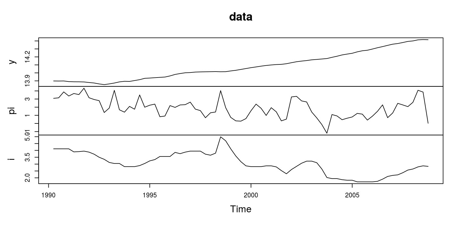
Over this sample period it would appear as if the natural logarithm of output might contain a deterministic time trend rather than a unit root. We can test for this by performing a unit root test, after removing the deterministic trend. To remove the deterministic trend we make use of the linear regression model. The trend will then pertain to the fitted values and the linear cyclical will be the difference between the fitted values and the original time series.
lin.mod <- lm(y ~ time(y))
lin.trend <- lin.mod$fitted.values
linear <- ts(lin.trend, start = c(1990, 2), frequency = 4)
lin.cycle <- y - linear
We can then apply the Augmented Dickey-Fuller test, that includes neither a time trend nor a constant (as both of these have been removed in the above linear regression).
adf.lin <- ur.df(lin.cycle, type = "none", selectlags = c("AIC"))
summary(adf.lin)
##
## ###############################################
## # Augmented Dickey-Fuller Test Unit Root Test #
## ###############################################
##
## Test regression none
##
##
## Call:
## lm(formula = z.diff ~ z.lag.1 - 1 + z.diff.lag)
##
## Residuals:
## Min 1Q Median 3Q Max
## -0.0102377 -0.0032151 -0.0009086 0.0033807 0.0110624
##
## Coefficients:
## Estimate Std. Error t value Pr(>|t|)
## z.lag.1 -0.04125 0.01635 -2.523 0.0139 *
## z.diff.lag 0.66969 0.08318 8.051 1.34e-11 ***
## ---
## Signif. codes:
## 0 '***' 0.001 '**' 0.01 '*' 0.05 '.' 0.1 ' ' 1
##
## Residual standard error: 0.004759 on 71 degrees of freedom
## Multiple R-squared: 0.5155, Adjusted R-squared: 0.5018
## F-statistic: 37.77 on 2 and 71 DF, p-value: 6.748e-12
##
##
## Value of test-statistic is: -2.5227
##
## Critical values for test statistics:
## 1pct 5pct 10pct
## tau1 -2.6 -1.95 -1.61In this case the results suggest that we are able to reject the null of a unit root at the 5% level. As the test statistic -2.5227 is smaller (i.e. more negative) than-1.95.
We can then plot the graph for the linear cycle in output.
par(mfrow = c(1, 1), mar = c(2.2, 2.2, 1, 1), cex = 0.6)
plot.ts(lin.cycle)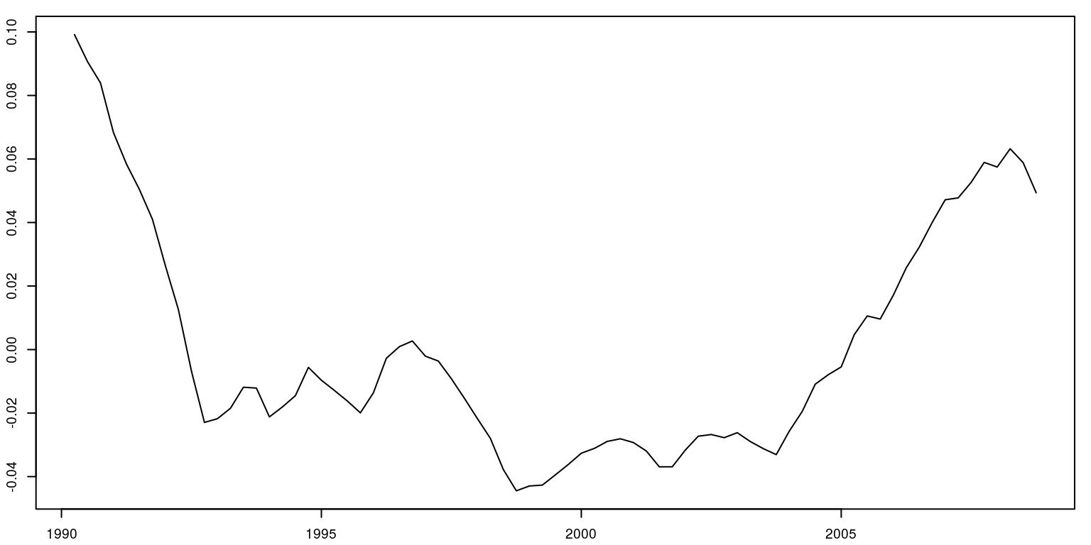
As there would appear to be a relatively sharp dip in 1992 and a flat section at the end in 2008, we include exogenous dummy variables for these periods.
dum92 <- rep(0, length(y))
dum92[11] <- 1
dum08 <- rep(0, length(y))
dum08[75] <- 1

dum92 <- ts(dum92, start = c(1990, 2), freq = 4)
dum08 <- ts(dum08, start = c(1990, 2), freq = 4)
dum <- cbind(dum92, dum08)
colnames(dum) <- c("dum92", "dum08")
1.1 Model estimation - with standard form of Cholesky decomposition
Note that the object data has the variables in the following order \((y,pi,i)\). After making use of a Cholesky decomposition on the matrix of contemporaneous parameters, this would imply:
- Only shocks to output can shift output contemporaneously.
- Only shocks to output and inflation can shift inflation contemporaneously.
- All shocks can affect the interest rate contemporaneously.
This ordering is consistent with macroeconomic theory and often applied in a closed-economy setting. Note also that instead of using the linear cycle, we’re going to use the natural logarithm of GDP. This would imply that we would need to include a deterministic trend in the model, to account for this time trend.
We can make use of information criteria to determine lag length for the VAR(\(p\)) model.
info.var <- VARselect(data, lag.max = 12, type = "both")
info.var$selection
## AIC(n) HQ(n) SC(n) FPE(n)
## 3 1 1 3Using the SIC/BIC these results suggest that we should make use of a VAR(\(1\)). We then need to estimate the reduced-form VAR to get an appropriate object that is to be manipulated into the structural-form of the model. Note that we have included a deterministic time trend and a constant in this model, where type="both", and the exogenous dummies.
var.est1 <- VAR(data, p = 1, type = "both", season = NULL,
    exog = dum)
summary(var.est1)
##
## VAR Estimation Results:
## =========================
## Endogenous variables: y, pi, i
## Deterministic variables: both
## Sample size: 74
## Log Likelihood: 225.491
## Roots of the characteristic polynomial:
## 0.9151 0.9151 0.4505
## Call:
## VAR(y = data, p = 1, type = "both", exogen = dum)
##
##
## Estimation results for equation y:
## ==================================
## y = y.l1 + pi.l1 + i.l1 + const + trend + dum92 + dum08
##
## Estimate Std. Error t value Pr(>|t|)
## y.l1 0.9509724 0.0186379 51.024 < 2e-16 ***
## pi.l1 0.0001075 0.0006596 0.163 0.871072
## i.l1 -0.0040457 0.0010918 -3.706 0.000429 ***
## const 0.6930124 0.2568211 2.698 0.008808 **
## trend 0.0004313 0.0001484 2.905 0.004967 **
## dum92 -0.0128255 0.0049238 -2.605 0.011313 *
## dum08 -0.0091503 0.0052170 -1.754 0.084012 .
## ---
## Signif. codes:
## 0 '***' 0.001 '**' 0.01 '*' 0.05 '.' 0.1 ' ' 1
##
##
## Residual standard error: 0.004806 on 67 degrees of freedom
## Multiple R-Squared: 0.9993, Adjusted R-squared: 0.9992
## F-statistic: 1.528e+04 on 6 and 67 DF, p-value: < 2.2e-16
##
##
## Estimation results for equation pi:
## ===================================
## pi = y.l1 + pi.l1 + i.l1 + const + trend + dum92 + dum08
##
## Estimate Std. Error t value Pr(>|t|)
## y.l1 9.94608 3.32134 2.995 0.003848 **
## pi.l1 0.44129 0.11754 3.754 0.000366 ***
## i.l1 -0.14781 0.19456 -0.760 0.450106
## const -135.05543 45.76638 -2.951 0.004362 **
## trend -0.08938 0.02645 -3.379 0.001217 **
## dum92 -1.20743 0.87743 -1.376 0.173377
## dum08 -2.88869 0.92968 -3.107 0.002770 **
## ---
## Signif. codes:
## 0 '***' 0.001 '**' 0.01 '*' 0.05 '.' 0.1 ' ' 1
##
##
## Residual standard error: 0.8565 on 67 degrees of freedom
## Multiple R-Squared: 0.5156, Adjusted R-squared: 0.4722
## F-statistic: 11.89 on 6 and 67 DF, p-value: 4.889e-09
##
##
## Estimation results for equation i:
## ==================================
## i = y.l1 + pi.l1 + i.l1 + const + trend + dum92 + dum08
##
## Estimate Std. Error t value Pr(>|t|)
## y.l1 0.202073 0.885476 0.228 0.8202
## pi.l1 0.073048 0.031337 2.331 0.0228 *
## i.l1 0.882880 0.051871 17.021 <2e-16 ***
## const -2.556297 12.201416 -0.210 0.8347
## trend -0.002151 0.007052 -0.305 0.7613
## dum92 -0.166469 0.233926 -0.712 0.4792
## dum08 -0.179153 0.247855 -0.723 0.4723
## ---
## Signif. codes:
## 0 '***' 0.001 '**' 0.01 '*' 0.05 '.' 0.1 ' ' 1
##
##
## Residual standard error: 0.2284 on 67 degrees of freedom
## Multiple R-Squared: 0.9221, Adjusted R-squared: 0.9151
## F-statistic: 132.1 on 6 and 67 DF, p-value: < 2.2e-16
##
##
##
## Covariance matrix of residuals:
## y pi i
## y 2.310e-05 0.0001804 2.515e-05
## pi 1.804e-04 0.7336510 1.086e-01
## i 2.515e-05 0.1086429 5.215e-02
##
## Correlation matrix of residuals:
## y pi i
## y 1.00000 0.04382 0.02291
## pi 0.04382 1.00000 0.55545
## i 0.02291 0.55545 1.00000Note the coefficients clearly show that we have included both a time trend and a constant, while the variance-covariance of the residuals shows that we have included covariance terms in the reduced-form model.
To set-up the matrix for the contemporaneous coefficients, we need to make use of a matrix that has the appropriate dimensions. This is easily achieved with the aid of the diagnol matrix. To code this appropriately we need to insert zeros for restrictions and NA in all those places that would not pertain to a restriction. Hence,
a.mat <- diag(3)
diag(a.mat) <- NA
a.mat[2, 1] <- NA
a.mat[3, 1] <- NA
a.mat[3, 2] <- NA
print(a.mat)
## [,1] [,2] [,3]
## [1,] NA 0 0
## [2,] NA NA 0
## [3,] NA NA NAFrom the printout, we see that we have imposed three restrictions in the top triangle, which would satisfy, \([(K^2 - K)/2]\), where \(K = 3\) in this case.
We then need to set-up the matrix for the identification of individual shocks. Once again starting with the diagnol matrix, we need to insert zeros into the covariance terms, while the variance for each of the individual shocks is to be retrieved. Hence,
b.mat <- diag(3)
diag(b.mat) <- NA
print(b.mat)
## [,1] [,2] [,3]
## [1,] NA 0 0
## [2,] 0 NA 0
## [3,] 0 0 NAThis printout suggest that there will be no covariance terms for the residuals. We are finally at a point where we can estimate the SVAR(1) model. This is achieved by including the the above two matrices. The maximum number of iterations has also been obtained, and we are also going to populate values for the Hessian, which is useful when looking to trouble shoot.
svar.one <- SVAR(var.est1, Amat = a.mat, Bmat = b.mat, max.iter = 10000,
    hessian = TRUE)
svar.one
##
## SVAR Estimation Results:
## ========================
##
##
## Estimated A matrix:
## y pi i
## y 1.00000 0.0000 0
## pi -7.80899 1.0000 0
## i 0.06796 -0.1481 1
##
## Estimated B matrix:
## y pi i
## y 0.004806 0.0000 0.0000
## pi 0.000000 0.8557 0.0000
## i 0.000000 0.0000 0.1899The results would suggest that both matrices have the correct functional form.
1.2 Impulse response functions
We can now proceed with the generation of the impulse response functions. The first of these considers the response of interest rates to an individual interest rate shock.
one.int <- irf(svar.one, response = "i", impulse = "i",
    n.ahead = 40, ortho = TRUE, boot = TRUE)
par(mfrow = c(1, 1), mar = c(2.2, 2.2, 1, 1), cex = 0.6)
plot(one.int)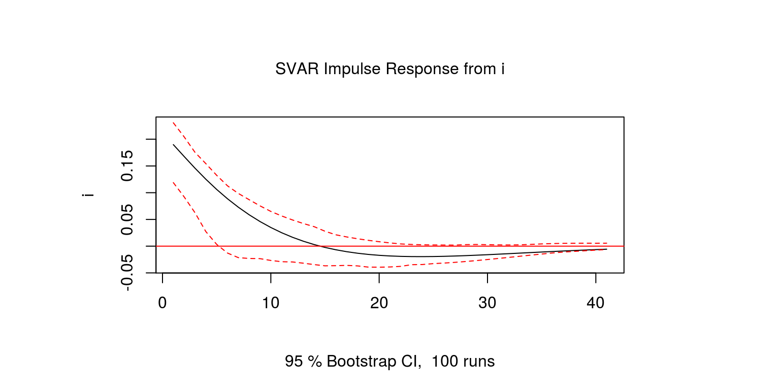
Note that as is to be expected, interest rate shocks are relatively persistent. The response of output to an interest rate shock could then be generated.
one.gdp <- irf(svar.one, response = "y", impulse = "i",
    n.ahead = 40, ortho = TRUE, boot = TRUE)
par(mfrow = c(1, 1), mar = c(2.2, 2.2, 1, 1), cex = 0.6)
plot(one.gdp)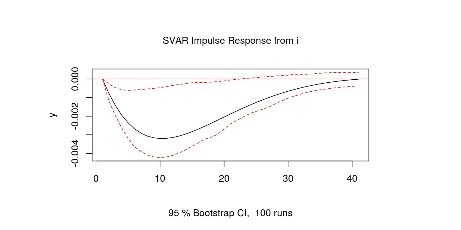
In this case, output declines following an interest rate shock. However, as the upper confidence interval remains at a value of zero, it would imply that the effect of the shock may not be significantly different from zero. Then lastly we consider the effect of the interest rate shock on inflation.
one.inf <- irf(svar.one, response = "pi", impulse = "i",
    n.ahead = 40, ortho = TRUE, boot = TRUE)
par(mfrow = c(1, 1), mar = c(2.2, 2.2, 1, 1), cex = 0.6)
plot(one.inf)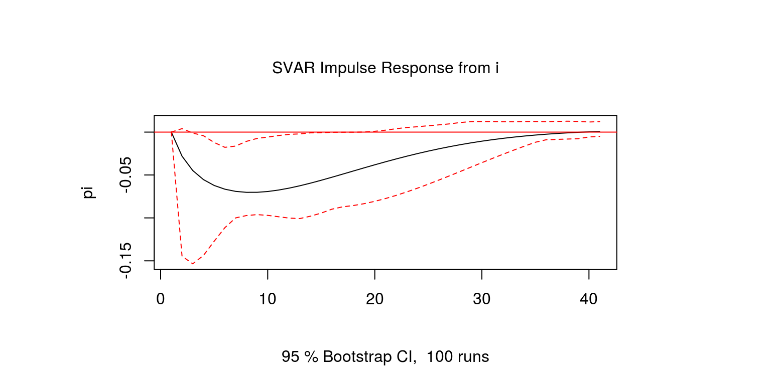
Similar to the previous case, inflation would also decline in reponse to an interest rate shock. However, the confidence intervals are relatively large once again.
Hence, these impulse response functions suggest that a contractionary monetary policy shock:
- increases the interest rate temporarily
- has a temporary negative effect on GDP
- has a temporary negative effect on inflation
This is consistent with theory, although the decline in inflation is greater than decline in output.
2 Using long-run restrictions for the aggregate demand and supply shocks
In the second example we will make use of a structural VAR with long-run restrictions to consider the effects of demand and supply side shocks, as in Blanchard & Quah (1989). The first few lines of the code complete the housekeeping by clearing the variables from the global environment while also closing all the graphics files.
rm(list = ls())
graphics.off()
We’re going to make use of the package vars once again, which you would have installed previously.
library(vars)Thereafter, we set the working directory, which should be where the data file is located. Note that to display the current working directory, one could use the command getwd().
setwd("C:\\Users\\image")This allows us to load the data into the data.frame, which has been called dat. This dataset contains postwar quarterly data for real GNP and the unemployment rate over the period 1950q2 - 1987q4.
after allowing for a trend break in output in 1973q4.
dat <- read.csv("BQdata.csv")The next chunk of code creates separate objects for each of the variables. The respective objects are GNP82 and USUNRATEE for real output and unemplotment rate. We take the first difference of output and remove the first observation of unemployment. The data is then demeaned in this case (which is slightly different to what Blanchard & Quah (1989), we they regressed out the mean and the time trend with a linear regression.
yt <- 100 * log(dat$GNP82)
dyt <- diff(yt)
unt <- dat$USUNRATEE[-1]

dyt <- dyt - mean(dyt)
unt <- unt - mean(unt)
Thereafter, we create time series objects for each variable, which are column binded in a single object vardat0. To ensure that there is no obvious error, we then plot the two variables in the object.
dyt <- ts(dyt, start = c(1951, 2), frequency = 4)
unt <- ts(unt, start = c(1951, 2), frequency = 4)
vardat0 <- cbind(dyt, unt)

plot.ts(vardat0, main = "")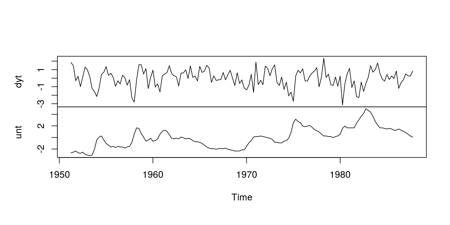
As in Blanchard & Quah (1989) we then estimate a bivariate VAR(8) model.
model0 <- VAR(vardat0, p = 8, type = "none")
summary(model0)
##
## VAR Estimation Results:
## =========================
## Endogenous variables: dyt, unt
## Deterministic variables: none
## Sample size: 139
## Log Likelihood: -163.62
## Roots of the characteristic polynomial:
## 0.929 0.8173 0.8173 0.8065 0.8065 0.8033 0.8033 0.7621 0.7621 0.7501 0.7501 0.6983 0.6983 0.6857 0.6268 0.2432
## Call:
## VAR(y = vardat0, p = 8, type = "none")
##
##
## Estimation results for equation dyt:
## ====================================
## dyt = dyt.l1 + unt.l1 + dyt.l2 + unt.l2 + dyt.l3 + unt.l3 + dyt.l4 + unt.l4 + dyt.l5 + unt.l5 + dyt.l6 + unt.l6 + dyt.l7 + unt.l7 + dyt.l8 + unt.l8
##
## Estimate Std. Error t value Pr(>|t|)
## dyt.l1 0.12774 0.11687 1.093 0.27655
## unt.l1 -0.61344 0.35630 -1.722 0.08763 .
## dyt.l2 0.24336 0.12489 1.949 0.05363 .
## unt.l2 1.71605 0.53622 3.200 0.00175 **
## dyt.l3 0.12233 0.12903 0.948 0.34497
## unt.l3 -0.73341 0.55831 -1.314 0.19142
## dyt.l4 0.15049 0.13081 1.150 0.25219
## unt.l4 0.35622 0.55085 0.647 0.51906
## dyt.l5 0.10930 0.13113 0.834 0.40613
## unt.l5 -0.62963 0.55189 -1.141 0.25614
## dyt.l6 0.25817 0.13191 1.957 0.05259 .
## unt.l6 0.62177 0.54634 1.138 0.25731
## dyt.l7 0.18209 0.13297 1.369 0.17337
## unt.l7 -0.42831 0.53666 -0.798 0.42634
## dyt.l8 -0.03629 0.10559 -0.344 0.73163
## unt.l8 -0.15982 0.34489 -0.463 0.64391
## ---
## Signif. codes:
## 0 '***' 0.001 '**' 0.01 '*' 0.05 '.' 0.1 ' ' 1
##
##
## Residual standard error: 0.9261 on 123 degrees of freedom
## Multiple R-Squared: 0.2873, Adjusted R-squared: 0.1946
## F-statistic: 3.099 on 16 and 123 DF, p-value: 0.0002015
##
##
## Estimation results for equation unt:
## ====================================
## unt = dyt.l1 + unt.l1 + dyt.l2 + unt.l2 + dyt.l3 + unt.l3 + dyt.l4 + unt.l4 + dyt.l5 + unt.l5 + dyt.l6 + unt.l6 + dyt.l7 + unt.l7 + dyt.l8 + unt.l8
##
## Estimate Std. Error t value Pr(>|t|)
## dyt.l1 -0.15666 0.03796 -4.127 6.71e-05 ***
## unt.l1 1.24740 0.11571 10.780 < 2e-16 ***
## dyt.l2 -0.11125 0.04056 -2.743 0.00700 **
## unt.l2 -0.56894 0.17414 -3.267 0.00141 **
## dyt.l3 -0.09507 0.04190 -2.269 0.02502 *
## unt.l3 0.10128 0.18131 0.559 0.57744
## dyt.l4 -0.04435 0.04248 -1.044 0.29850
## unt.l4 -0.06988 0.17889 -0.391 0.69676
## dyt.l5 -0.02006 0.04258 -0.471 0.63837
## unt.l5 0.23752 0.17923 1.325 0.18756
## dyt.l6 -0.11380 0.04284 -2.657 0.00894 **
## unt.l6 -0.14020 0.17743 -0.790 0.43095
## dyt.l7 -0.04587 0.04318 -1.062 0.29019
## unt.l7 0.09310 0.17428 0.534 0.59419
## dyt.l8 0.03612 0.03429 1.053 0.29424
## unt.l8 0.03951 0.11201 0.353 0.72489
## ---
## Signif. codes:
## 0 '***' 0.001 '**' 0.01 '*' 0.05 '.' 0.1 ' ' 1
##
##
## Residual standard error: 0.3008 on 123 degrees of freedom
## Multiple R-Squared: 0.9708, Adjusted R-squared: 0.967
## F-statistic: 255.7 on 16 and 123 DF, p-value: < 2.2e-16
##
##
##
## Covariance matrix of residuals:
## dyt unt
## dyt 0.8529 -0.1754
## unt -0.1754 0.0896
##
## Correlation matrix of residuals:
## dyt unt
## dyt 1.0000 -0.6345
## unt -0.6345 1.0000Thereafter, we apply the long-run restrictions, by making use of the BQ command.
model1 <- BQ(model0)
summary(model1)
##
## SVAR Estimation Results:
## ========================
##
## Call:
## BQ(x = model0)
##
## Type: Blanchard-Quah
## Sample size: 139
## Log Likelihood: -180.619
##
## Estimated contemporaneous impact matrix:
## dyt unt
## dyt 0.66506 -0.6445
## unt 0.02376 0.2998
##
## Estimated identified long run impact matrix:
## dyt unt
## dyt 0.6972 0.00
## unt -5.9859 4.98
##
## Covariance matrix of reduced form residuals (*100):
## dyt unt
## dyt 85.77 -17.742
## unt -17.74 9.045To extract the standard impulse response functions for shocks from each variable, we could then make use of the command irf.
irf.dyt <- irf(model1, impulse = "dyt", boot = FALSE, n.ahead = 40)
irf.unt <- irf(model1, impulse = "unt", boot = FALSE, n.ahead = 40)
We can then create an object for the cumulative impulse response functions for the supply shocks
supply <- cbind(cumsum(irf.dyt$irf$dyt[, 1]), irf.dyt$irf$dyt[,
    2])
Similarly, to get the cummulative effect of demand shocks we need the cumulative sum and to match the results in Blanchard & Quah (1989) we consider the effects of a negative demand side shock and multiply through by -1
demand <- cbind(-1 * cumsum(irf.unt$irf$unt[, 1]), -1 *
    irf.unt$irf$unt[, 2])
We can then plot the impulse response functions for the demand shock as follows:
plot.ts(demand[, 1], col = "black", lwd = 2, ylab = "",
    xlab = "", main = "Demand Shock", xlim = c(0, 40), ylim = c(-0.6,
        1.4))
lines(demand[, 2], col = "blue", lwd = 2)
abline(h = 0)
legend(x = "topright", c("Output response", "Unemployment response"),
    col = c("black", "blue"), lwd = 2, bty = "n")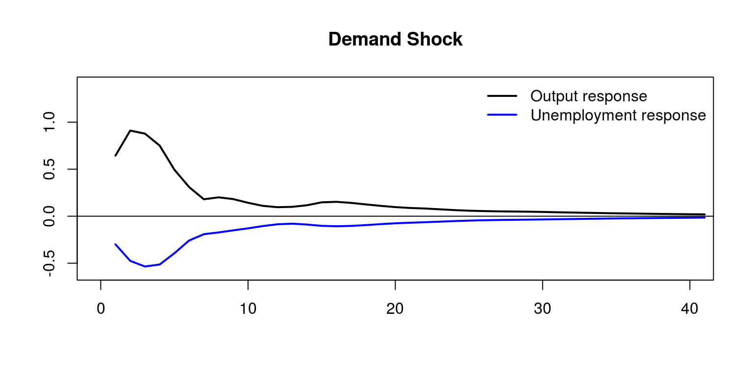
where we note that transitory (demand) shocks have no long-run impact on the level of output or unemployment. Similarly, the effect of a supply side shock would look as follows:
plot.ts(supply[, 1], col = "black", lwd = 2, ylab = "",
    xlab = "", main = "Supply Shock", xlim = c(0, 40), ylim = c(-0.6,
        2))
lines(supply[, 2], col = "blue", lwd = 2)
abline(h = 0)
legend(x = "topright", c("Output response", "Unemployment response"),
    col = c("black", "blue"), lwd = 2, bty = "n")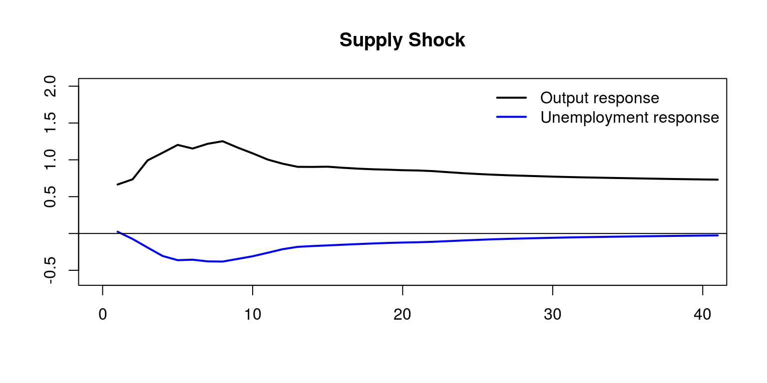
However, permanent (supply) shocks have a long-run impact on the level of output but not on the level of unemployment.
This would allow one to conlcude that demand shocks have humped shape effects on output and unemployment that vanishes after 3 years, while supply shocks have permanent effect on output after 5 years. In addition, demand shocks contribute substantially to output variability in the short run.